AN BRIEF INTRODUCTION TO EXTREME VALUE THEORY
11th, February, 2019
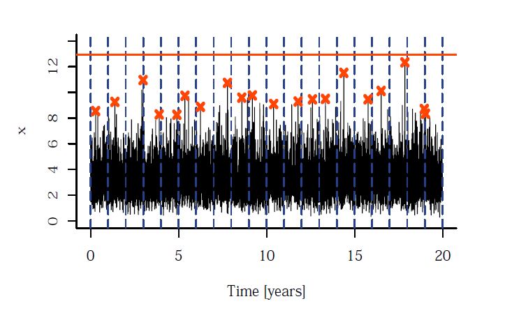
Flooding can occur in two different ways. Whenever there is too much extra water accumulated over long period in a river's channel because of rain, ice melting which can result in breaking through the river bank and spreading over the land. Other natural disasters such as hurricanes, cyclones, earthquakes etc. can cause flooding immediately and very heavily. In the latter case it is a big observation that causes flooding, which means that partial maxima exceed some threshold. In fact, this kind of intellectual curiosity has motivated the development of the theory of extremes.

The target is to find the limit distributions for the maxima of independent and identically distributed random variables.
Assume that \(X_1, X_2, …, X_n\) IID variables and let F be the underlying distribution function.
We define \(x^*\) is the right endpoint of F, which may be infinite, like
$$x^* := \sup \{ x: F(x) <1 \} $$
Then,
$$ \max(X_1, X_2, …, X_n) \rightarrow^P x^* , \ \ n \rightarrow \infty$$
where \( \rightarrow^P \) means convergence in probability or
$$ P(\max(X_1, X_2, …, X_n) \leq x) = P(X_1 \leq x, X_2 \leq x, …, X_n \leq x) = F^n(x), $$
which tends to 0 for \( x < x^*\) and to 1 for \( x \geq x^*\) as n tends to \( \infty\). Therefore, a normalization is necessary to obtain a nondegenerate limit distribution.
Suppose there exists a sequence of constants \(a_n\ >0\), and \( b_n \in \mathbb{R}\) (n = 1,2, …), such as
$$\displaystyle \lim_{n \rightarrow \infty} P( \frac{\max(X_1, X_2, …, X_n) – b_n}{a_n} \leq x) = \displaystyle \lim_{n \rightarrow \infty} F^n(a_n x +b_n) = G(x) \ \ (1)$$
and G(x) is a nondegenerate distribution function for every continuity point x of G. These distributions are called extreme value distributions.
So the question now is whether or not such a sequence of constant \( a_n, b_n\), G nondegenerate distribution function exist. And for each of the G function, what is the necessary and sufficient conditions on the initial distribution F such that the above equation (1) holds or simply finding the (maximum ) domain of attraction of G, which means the class of distribution F.
By taking logarithms, we get the equivalent relation for (1) as following:
$$ \lim_{n \rightarrow \infty} n \log F(a_nx + b_n) = log G(x), \quad (2)$$
for each continuity point x where \(0 < G(x) <1\).
Then it follows that \(F(a_n x+b) \rightarrow 1\) as \( n \rightarrow \infty\) for each such x.
Therefore,
$$ \displaystyle \lim_{n \rightarrow \infty} \frac{-\log F(a_n x + b_n)}{1-F(a_n x+b_n)} = 1, \ (3)$$
From (2) and (3), we get
$$ \displaystyle \lim_{n \rightarrow \infty} n(1- F(a_n x+b_n) ) = -logG(x). $$
Theorem 1: Let \(a_n >0\) and b_n be real sequences of constants and G a nondegenerate distribution function. The following statements are equivalent:
1. For each continuity point x of G,
$$ \displaystyle \lim_{n \rightarrow \infty} F^n(a_n x+b_n) = G(x)$$
2. For each continuity point x of G for which 0 < G(x) <1,
$$ \displaystyle \lim_{t \rightarrow \infty}t(1- F^n(a_{[t]} x+b_{[t]}) = - logG(x)$$
3. For each continuity point x of \(D (x) = G^{\leftarrow}(\exp(-1/x))\) (*),
$$ \displaystyle \lim_{n \rightarrow \infty} \frac{U(tx) –b_{[t]}}{a_{[t]}} = D(x).$$
Note *: \(f^{\leftarrow}\) be the left-continuous inverse of any nondecreasing function f, i.e.,
$$ f^{\leftarrow} (x) = \inf \{ y: f(y) \geq x \}. $$
Theorem 2: (Fisher and Tippet (1928), Gnedenko (1943)) The class of extreme value distributions is \( G_{\gamma}(ax+b) \) with a >0, b real where
$$ G_{\gamma}(x) = \exp(- (1+\gamma x)^{-1/\gamma} ), \ 1+ \gamma x >0,$$
With \( \gamma \) real, which is called the extreme value index and where for \( \gamma =0\) the right-hand side is \( \exp( - e^{-x}) \).
The proof idea is by using the previous theorem, to check the third condition, which equivalent to the first condition, or the definition of the extreme value distributions.
Let see a small application of this. Whether there is limited life span for humans?
If we consider the life span of human as random, how its probability distribution’s right endpoint looks like? Is it finite or infinite? How the problem can be considered from the point of view of extreme value theory?
Note that, considering the subclasses \( \gamma >0, \gamma = 0, \text{ and} \ \gamma <0 \) of \( G_{\gamma}(x)\) separately:
(1), For \( \gamma >0 \), it follows \( G_{\gamma}(x) <1\) for all x, i.e., the right endpoint of distribution is infinity.
(2), For \( \gamma = 0 \), it follows \( G_{\gamma}(x) \sim 1 - \exp(-x) \text{as} x \rightarrow \infty \), i.e., the right endpoint of distribution is infinity.
(3), For \( \gamma <0 \), it follows \(1 - G_{\gamma}(- \gamma^{-1} –x ) \sim (-yx)^{-1/\gamma}\) as \( x \rightarrow 0\), i.e., the right endpoint of distribution is \(- \gamma^{-1}\).
Back to the life span of humans, we can test equivalently whether the extreme value index is negative by testing hypothesis:
$$ H_0 : \gamma \geq 0 \ \text{versus} \ H_1: \gamma <0.$$
There is a data set consists of the total lifespan (in days) of about 10 391 people born in Netherlands in the years 1877 – 1881, still alive on January 1, 1971, and who died as a resident of the Netherlands.
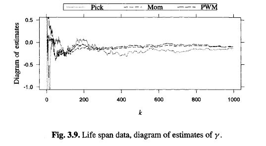
This is a diagram of estimates for the Pickands, moment, and probability-weighted moment estimators. For practical all k, the null hypothesis is rejected. Therefore, for the given data set, the hypothesis \( \gamma <0 \) is not rejected. It means that we have \( \displaystyle \lim_{t \rightarrow \infty} U(t) < \infty \). Hence, we shall believe that there is an age that cannot be exceeded. How we can estimate the maximal age? Using the limit relation of theorem 1, we have
$$ \frac{U(tx) – U(t)}{a_{[t]}} \rightarrow \frac{x^{\gamma} -1}{\gamma}, \ \ \text{as} \ t \rightarrow \infty,$$
Let \( x = \infty\) (valid for \(\gamma <0 \)), we get
$$ \frac{U(\infty) – U(t)}{a_{[t]}} \rightarrow \frac{x^{\gamma} -1}{\gamma}, \ \ \text{as} \ t \rightarrow \infty,$$
Or
$$U (\infty) \approx \displaystyle \lim_{t \rightarrow \infty} U(t) - \frac{a_{[t]}}{\gamma}. $$
This relation will be the basis to estimate the maximal age of life span.
Reference:
(1) Extreme Value Methods and their Applications: Predicting the Unpredictable. Jonathan Tawn
(2) Extreme Value Theory An Introduction, Laurens De Haan Ana Ferreira.