V Quantum Computation

The discussion in Section III implies that quantum computers can achieve, at least, the same tasks as a classical computer. Since this requires reversible logics, we first illustrate this by an example, namely, the computation of the sum of two numbers.

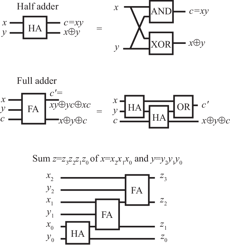
Binary numbers can be added just like decimal numbers, bit by bit starting with the least significant bits, and carrying over bits to the next more significant bit. Consider, e.g., the sum $3+3$, which in binary code is $11+11$. We first add the last two bits (i.e., the least significant bits), resulting in $1+1=10$. The last bit of this (0) is the last bit of our result, while the first bit needs to be carried over. We then add the first two bits, and to this the carry-on bit, giving $1+1+1=11$. This again results in a carry-on bit. There are no further bits to be processed, so the carry-on bit becomes the most significant bit. Our result now has three bits: 110, which is the same as $4+2+0=6$.

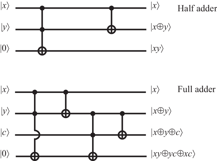
In classical computers, these operations can be carried out using half-adder and full-adder components, which can be realized using elementary binary gates as shown in Fig. 10. Because of $x+y=y+x$, the depicted circuit is irreversible (furthermore, it requires to copy bits). Figure 11 shows that the same operations can also be achieved quantum mechanically using a combination of reversible CNOT and CCNOT gates, which generate additional outputs that can be used to reverse the calculation.

Adding two numbers with reversible gates does not increase the efficiency of the algorithm. This is in contrast to the following examples, which concern true quantum algorithms that solve specific tasks more efficiently than classical algorithms.

Efficient quantum algorithms generally exploit the quantum parallelism to carry out many calculations in one step, which is particularly useful if one is interested in a global property of these calculations. This is nicely illustrated by the Deutsch-Josza algorithm, which allows to establish a specific feature of certain Boolean functions $f:x\to \{0,1\}$ that specifically fall into one of the following two classes: either the function is constant (i.e., the output bit $f$ is either always 1, or always 0), or it is balanced (i.e., the output bit is 0 for one half of the input values, and 1 for the remaining half).

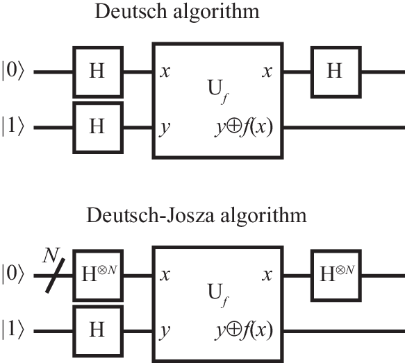
Assume that we are given a function $f(x)$ which is guaranteed to be either constant or balanced, but at the outset we do not know to which of the two classes it belongs. Classically, we need at least two function evaluations to find out that a function is balanced—and this is only in the fortunate case that we immediately pick two inputs for which the outputs differ. In order to certify that a function is constant we need $2^N/2+1=2^{N-1}+1$ function evaluations—that’s because if the function is balanced, we may by chance first pick $2^N/2$ inputs that all result in the same output. In contrast, using quantum gates, the Deutsch-Josza algorithm, shown in Fig. 12, requires only a single function evaluation to determine whether the function is constant or balanced. (The upper panel of the figure shows the Deutsch algorithm, the special case of a function $f(x)$ with single-bit input, which is addressed on worksheet 3.)

Starting from the initial state $|{\psi }_0⟩=|0\mathrm{\dots }001⟩$, Hadamard gates are used to form the superposition

$$|{\psi }_1⟩=\prod _n{H}_n|{\psi }_0⟩=2^{-N/2}\sum _x|x⟩\frac{|0⟩-|1⟩}{\sqrt{2}}=|\mathrm{\Psi }⟩\frac{|0⟩-|1⟩}{\sqrt{2}}$$

(see also Fig. 6(b)). If $f(x)=1$, the function gate changes the state of the last qubit into $\frac{|1⟩-|0⟩}{\sqrt{2}}=-\frac{|0⟩-|1⟩}{\sqrt{2}}$; for $f(x)=0$, the state of this qubit remains $\frac{|0⟩-|1⟩}{\sqrt{2}}$. Therefore, the function gate introduces factors ${(-1)}^{f(x)}$ in front of each basis state $|x⟩$, resulting in

$$|{\psi }_2⟩=U_f|{\psi }_1⟩=2^{-N/2}\sum _x{(-1)}^{f(x)}|x⟩\frac{|0⟩-|1⟩}{\sqrt{2}}.$$

In the final step, Hadamard gates are applied to all but the last qubit. Using the result shown in Fig. 6(c), this delivers the final state

$$|{\psi }_3⟩=2^{-N}\sum _z\sum _x{(-1)}^{x\cdot z+f(x)}|z⟩\frac{|0⟩-|1⟩}{\sqrt{2}}.$$

Let us now have a look at the amplitude of the state with $|z⟩=|0⟩$, which is given by $2^{-N}{\sum }_x{(-1)}^{f(x)}$. If $f(x)$ is balanced, this amplitude vanishes. On the other hand, if $f(x)=c$ is constant, this amplitude takes the value $\pm 1$ (depending on whether $c=0$ or $c=1$). Therefore, if $f$ is constant, a measurement of all qubits will find them all taking the value $0$, while this will never happen if the function is balanced. Remarkably, using quantum parallelism, the distinction of both cases has been achieved with a single operation of the function gate.

A notable ingredient of the Deutsch-Josza is the introduction of conditional phase factors (such as ${(-1)}^{f(x)}$) in front of each of the computational basis states. This strategy is also at the core of the practically more important algorithms discussed next.

Grover’s quantum search algorithm exploits quantum parallelism to speed up the search for solutions among a large set of candidate solutions. A prime example is the search for entries in a database which match to a given key. Let us enumerate all entries by an integer index $x$, and assume for simplicity that the size of the database is $𝒩=2^N$. The entries matching the key can then be characterized by an oracle function $f(x)$, which is a Boolean function that returns $f(x)=1$ if entry $x$ matches to the key; otherwise, $f(x)=0$.

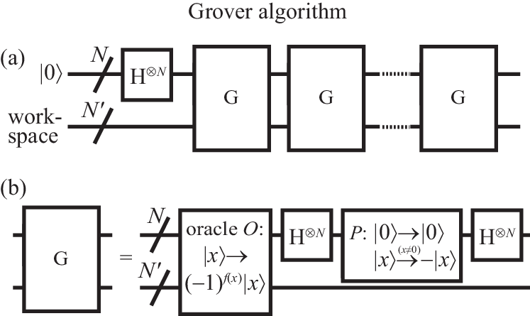
Assume that there are $ℳ\ll 𝒩$ entries matching the key. Classically, we need to make $\approx 𝒩/ℳ\gg 1$ queries of the database (or calls of the oracle function) to find one of these entries. The Grover algorithm, shown in Fig. 13, only requires $O(\sqrt{𝒩/ℳ})$ calls of the oracle function—not an exponential speedup, but still sizeable when the database is large.

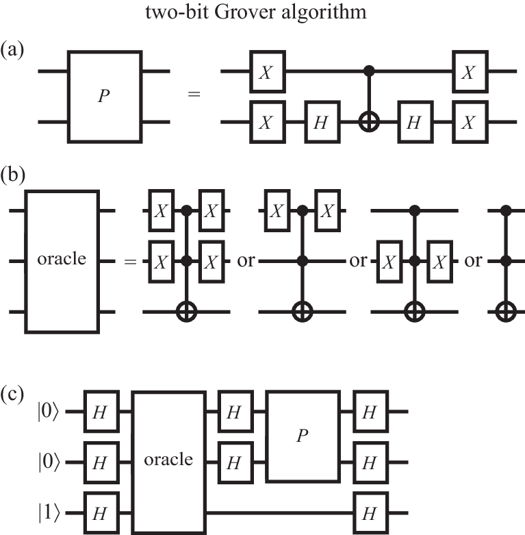
The first step initializes the index register in the now very familiar equal-superposition state $|\mathrm{\Psi }⟩$. This is followed by a sequence of operations $G$, known as the Grover iterate, in which the oracle gate $\widehat{O}$ is called once. Its action is defined to flip the phase of all solutions: $\widehat{O}|x⟩={(-1)}^{f(x)}|x⟩$. As we have seen in the Deutsch-Josza algorithm, this can be achieved with a function gate acting as ${\widehat{O}}_f|x⟩|q⟩=|x⟩|f(x)\oplus q⟩$, where the oracle qubit $q$ is initialized as $\sqrt{1/2}(|0⟩-|1⟩)$ (Fig. 13 reserves $N^{\prime }$ workspace qubits for the implementation of the oracle). The Grover iterate also contains a conditional phase gate $P=2|0⟩⟨0|-\widehat{I}$, which inverts the phase of all computational basis states with exception of the state $|0⟩$. This is embedded into Hadamard gates, resulting into

$$P^{\prime }=(\prod _n{H}_n)(2|0⟩⟨0|-\widehat{I})(\prod _n{H}_n)=2|\mathrm{\Psi }⟩⟨\mathrm{\Psi }|-\widehat{I}.$$

The Grover iterate can therefore be written as

$$G=(2|\mathrm{\Psi }⟩⟨\mathrm{\Psi }|-\widehat{I})\widehat{O}.$$

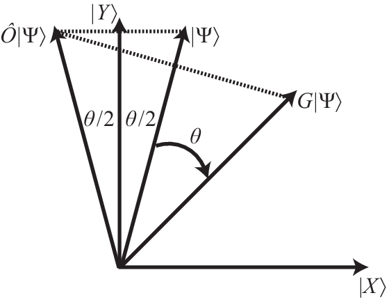
The purpose of the Grover iterate is to rotate the initial state into the direction of the equal superposition of solutions $|X⟩\equiv \frac{1}{\sqrt{ℳ}}{\sum }_{m=1}^{ℳ}|x_m⟩$, where we have enumerated all solutions as $x_m$, $m=1,2,3,\mathrm{\dots },ℳ$. This rotation takes place in a plane spanned by $|X⟩$ and $|Y⟩=\frac{1}{\sqrt{𝒩-ℳ}}{\sum }_{m=1}^{𝒩-ℳ}|y_m⟩$, the equal superposition of all non-solutions $y_m$, $m=1,2,3,\mathrm{\dots },𝒩-ℳ$. Figure 14 illustrates how this works. The initial state can be written as

$$|\mathrm{\Psi }⟩=\sqrt{ℳ/𝒩}|X⟩+\sqrt{1-ℳ/𝒩}|Y⟩,$$

and therefore lies in the $X$,$Y$ plane. The unit vector

$$\mathrm{\Psi }=(\sqrt{ℳ/𝒩},\sqrt{1-ℳ/𝒩})=(\sin \theta /2,\cos \theta /2)$$

can be parameterized in terms of the angle $\theta /2$ between $\mathrm{\Psi }$ and the $Y$ axis. For $ℳ\ll 𝒩$, $\theta =2\arccos \sqrt{1-ℳ/𝒩}\approx 2\sqrt{ℳ/𝒩}$ is small, such that $\mathrm{\Psi }$ is almost parallel to the $Y$ axis.

Per definition, the oracle function acts as

$$\widehat{O}(\alpha |X⟩+\beta |Y⟩)=-\alpha |X⟩+\beta |Y⟩,$$

which amounts to a reflection about the $Y$ axis. The phase gate $P^{\prime }$ performs another reflection, now about the $\mathrm{\Psi }$ axis. As a result, the state is rotated by an angle $\theta$ towards the $X$ axis. Repeating this rotation $\approx (\pi /4)\sqrt{𝒩/ℳ}$ times rotates the state vector close to the $X$ axis—the misalignment will be less than $\theta /2$. With high probability, a measurement of the final state will therefore deliver a solution $x_m$ of the search problem.

An instructive example is a two-bit search with one solution $x_1$, depicted in Fig. 15. Panel (a) shows a realization of the $P$ gate with $H$, $X$, and CNOT gates (as a matter of fact, this realizes $-P$, but an overall phase factor of a quantum state is non-detectable). Depending on the binary representation of $x_1$, the oracle function takes one of four possible forms, which can be implemented using Toffoli (CCNOT) and $X$ (NOT) gates as shown in panel (b). For $𝒩=4=2^2$, $ℳ=1$, the angle of the initial state vector $\mathrm{\Psi }$ with the $Y$ axis is $\theta /2={30}^{\circ }$. The Grover iterate rotates the state by $\theta ={60}^{\circ }$. A single iteration therefore rotates the state onto the $X$ axis, which immediately identifies the matching entry $x_1$. In contrast, a classical search would on average require $2.25$ oracle calls before the solution is found.

Consider the Fourier transformation

$$\tilde{f}(z)=2^{-N/2}\sum _{x=0}^{2^N-1}{\omega }^{xz}f(x)$$

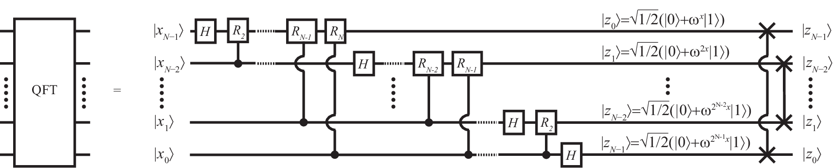
of an $N$-bit function $f$. Here, we abbreviated $\omega =e^{2\pi i/2^N}$, such that ${\omega }^{xz}=e^{2\pi ixz/2^N}$ (where $xz$ is an ordinary, not bitwise, multiplication). Classically, implementation of the Fourier transformation takes $O(2^N)$ elementary gate operations. In contrast, its quantum-mechanical analogue, the quantum Fourier transformation

$$U_{QFT}|x⟩=2^{-N/2}\sum _{z=0}^{2^N-1}{\omega }^{xz}|z⟩\equiv |\tilde{x}⟩,$$

can be implemented with $O(N^2)$ gate operations, which constitutes an exponential increase in efficiency that can be exploited in a range of algorithms.

The corresponding circuit is shown in Fig. 16. The verification that the depicted circuit computes the quantum Fourier transformation can be based on the product representation

$$|\tilde{x}⟩=|z_{N-1}⟩|z_{N-2}⟩\mathrm{\cdots }|z_0⟩,$$

where $|z_n⟩=\sqrt{1/2}(|0⟩+{\omega }^{2^{n}x}|1⟩)$. Because of the $2\pi$ periodicity of the phase, the phase factors can be written as ${\omega }^{2^{N-n}x}=e^{i2\pi 0.x_{n-1}{x}_{n-2}\mathrm{\cdots }{x}_0}$, where we introduced the binary fractions

$$x/2^n=\sum _{k=0}^{N-1}{x}_k{2}^{k-n}\equiv x_{N-1}\mathrm{\cdots }{x}_n.x_{n-1}\mathrm{\cdots }{x}_0$$

in a notation analogous to the one denoting fractional decimal numbers. As shown in the figure, the required transformation of each qubit can be achieved efficiently by first applying a Hadamard gate, followed by phase rotation gates

that are controlled by the less significant qubits.

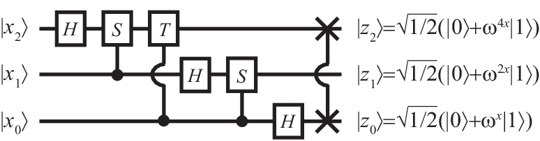
An instructive example is the three-bit quantum Fourier transformation, where $\omega =\exp (2\pi i/8)=\sqrt{i}$. In this case, $R_1=T$ is the $\pi /8$ gate, and $R_2=S$ is the phase gate. The corresponding circuit is shown in Fig. 17.

Phase estimation.—A key application of the quantum Fourier transformation is the estimation of the (reduced) phase $\varphi$ of an eigenvalue $\lambda =e^{2\pi i\varphi }$ of a unitary operator $U$, where . This can be used for a problem called order finding, which in itself is a central step in the prime factorization of numbers. Phase estimation can also be used for a problem know as quantum counting. These problems are briefly discussed later; at the moment it suffices to know that they involve different operators $U$.

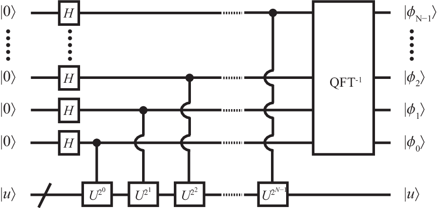
Given the eigenstate $|u⟩$ corresponding to $\lambda$, $\varphi$ can be estimated efficiently as an $N$ bit binary fraction $\varphi \approx 0.{\varphi }_{N-1}{\varphi }_{N-2}\mathrm{\cdots }{\varphi }_0$ using the circuit shown in Fig. 18. Since $U|u⟩=\lambda |u⟩$ and $\lambda ={\omega }^{2^N\varphi }$, where $\omega =e^{2\pi i/2^N}$, the controlled-$U^{2^n}$ operations in the first part of the algorithm transform the qubits into the state $\sqrt{1/2}(|0⟩+{\omega }^{2^n(2^N\varphi )}|1⟩)$. With $N$-bit precision, $2^N\varphi \approx {\varphi }^{\prime }$, where the integer number ${\varphi }^{\prime }$ has the $N$-bit representation ${\varphi }^{\prime }={\varphi }_{N-1}{\varphi }_{N-2}\mathrm{\cdots }{\varphi }_0$. The intermediate state can therefore be approximated by the product representation

$$|z_{N-1}⟩|z_{N-2}⟩\mathrm{\cdots }|z_0⟩=U_{QFT}|{\varphi }^{\prime }⟩=|{\tilde{\varphi }}^{\prime }⟩$$

of the Fourier-transformed $N$-bit estimate of $2^N\varphi$, whose binary digits ${\varphi }_n$ are then recovered by an inverse Fourier transformation.

Quantum counting.—A straightforward application of the phase estimation algorithm is the determination of the number $ℳ$ of solutions in an $𝒩$-item search problem, as encountered in the Grover search. In the $X$-$Y$ plane, the rotation by one Grover iteration can written as the

which is a unitary matrix with eigenvalues $e^{\pm i\theta }$. We also know that $|\mathrm{\Psi }⟩$ lies in the $X$-$Y$ plane, and therefore is a superposition of the two corresponding eigenstates, which can be fed into the slot for $|u⟩$.

Order finding.—Phase estimation can also be used to solve the following number-theoretic problem: given two numbers $a$ and $M$ without common divisors, what is the order $r$ of $a\mathrm{mod}M$, defined as the smallest positive integer $r$ such that $a^r\mathrm{mod}M=1$? Here, the modulo operation determines the remainder of the division by $M$. The order can be obtained by estimating the phase of the eigenvalues ${\lambda }_n=\exp (2\pi in/r)$ of the operator $U|x⟩=|ax\mathrm{mod}M⟩$ (for ; otherwise $U|x⟩=|x⟩$, which guarantees that $U$ is unitary). Conveniently, the sum of eigenfunctions

$$|u_n⟩=\frac{1}{\sqrt{r}}\sum _{z=0}^{r-1}\exp (-2\pi inz/r)|a^z\mathrm{mod}M⟩$$

is independent of $r$, ${\sum }_n|u_n⟩=|1⟩$. Therefore, initializing $|u⟩=|1⟩$, the phase estimation algorithm will deliver an approximation of $n/r$, where each value $n$ in the range appears with equal probability $1/r$. This suffices to reconstruct the order $r$ (most efficiently, by a method based on continued fractions).

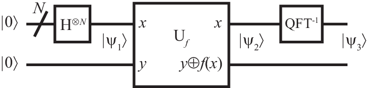
Period finding.—Note that the order $r$ is the period of the function $f(x)=a^x\mathrm{mod}M$, i.e., $f(x)=f(x+r)$. It is noteworthy that a variant of the procedure above can be used to find the period of any integer-valued function. The corresponding circuit is shown in Fig. 19. The indicated intermediate states are $|{\psi }_1⟩=|\mathrm{\Psi }⟩|0⟩$ and

$$|{\psi }_2⟩=2^{-N/2}\sum _{x=0}^{2^N-1}|x⟩|f(x)⟩=\frac{1}{\sqrt{r}}\sum _{n=0}^{r-1}|\widetilde{{(n/r)}^{\prime }}⟩|\widehat{f}(n)⟩,$$

where, as before, ${(n/r)}^{\prime }$ denotes the $N$-bit estimate of $2^N(n/r)$, and the tilde indicates the Fourier-transformed state. Furthermore, we abbreviated

$$|\widehat{f}(n)⟩=\frac{1}{\sqrt{r}}\sum _{x=0}^{r-1}\exp (-2\pi nix/r)|f(x)⟩.$$

The inverse Fourier transformation converts this into the final state

$$|{\psi }_3⟩=\frac{1}{\sqrt{r}}\sum _{n=0}^{r-1}|{(n/r)}^{\prime }⟩|\widehat{f}(n)⟩,$$

so that the measurement of the output qubits in the first register delivers an $N$-bit approximation of $2^N(n/r)$.

Prime factorization.—In a loose mathematical sense, the factors of an integer number $M$ can also be interpreted as ’periods’ of that number. Indeed, it turns out that the order-finding problem is equivalent to the problem of prime number factorization, and therefore can be solved efficiently using phase estimation. This is embodied in Shor’s factorization algorithm. Because the accurate description of this algorithm requires various number-theoretic concepts, we here only mention one key ingredient: assume we have randomly chosen a number $a$ and found that the order $r$ of $a\mathrm{mod}M$ is even (otherwise, start again with another randomly chosen $a$). Then $b=a^{r/2}$ is still an integer, which fulfills

$$b^2\mathrm{mod}M=1\Rightarrow (b+1)(b-1)\mathrm{mod}M=0.$$

Furthermore assume that $b\mathrm{mod}M\ne -1$ (otherwise, start again…). It then follows that $b_{+}=(b+1)$ or $b_{-}=(b-1)$ shares a nontrivial factor with $M$. The largest factor (the greatest common divisor, gcd) can be found efficiently using Euclid’s algorithm: given $c>d$, iterate the identity $\gcd (c,d)=\gcd (d,c\mathrm{mod}d)$ until the smaller number is a divisor of the larger number; the smaller number is then the gcd of $c$ and $d$, which delivers a factor of $M$.