INFINITE SERVER QUEUES THEORY
5 th February, 2019.
Queueing theory is the study of problems involving waiting or queueing and helps to analyse and understand the queueing behaviour and then, make decisions about the resources allocation or utilization.
We list some typical examples we might see every day:
- waiting for service in banks
- waiting supermarkets
- waiting for public transports
- waiting at a red light (cars)
- waiting for apps response in the mobile, computer
- etc.
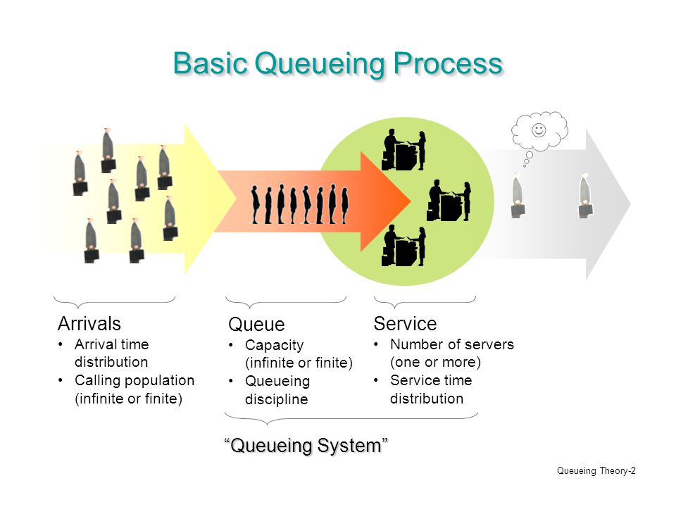 Queueing models consist of three main components:
- arrival process:
- how customers arrive such as singly or in groups.
- What are the distribution of the arrivals over time and interarrival time ( time between successive arrivals).
- Service pattern:
- which resources needed for serving customers and how many available servers in the system.
- The distribution of service time, i.e. how long each service will take.
- whether each server has a separate queue or all servers share the same queue.
- queue characteristics:
- Queueing rule, i.e. how customers waiting for service, e.g. FIFO (first-in-first-out), LIFO (last-in-first-out) or random.
- Have any priorities for "emergency" customers.
- Is there any case of
- balking (customers don’t join the queue since it is already too long)
- reneging (customers decide to leave the queue since they have waited too long for service)
- jockeying (customers switch between queues in order to get served faster),
Queueing models are often described in the form A/B/c using Kendall’s notation, where A indicates the arrival process, B indicates the service time distribution and c denotes the number of servers. This notation was used mainly for queueing models in continuous time rather than discrete time. For example, in continuous time, Poisson arrival process means a negative exponential distribution for interarrival times, whereas in discrete time Poisson arrivals simply means that the number of arrivals at
a particular time is Poisson distributed. Other notations can be used for discrete time models \(A_D/B_D/c\) where \(A_D\) indicates the distribution of number of arrivals at a discrete time point, and \(B_D\) denotes the discrete distribution of service time. -
Common options for A and B are:
- M: a Poisson arrival process or a exponential distribution for service time.
- D: deterministic or constant value.
- G: a general distribution.
Infinite server models is a type of queueing models which assume there are an unlimited supply of servers. When modelling systems by the infinite server assumption, all arrivals are honoured i.e. customers get served immediately upon arrival without waiting. As a result, customers are mutually independent.
Unlike many capacitated models, infinite server models can produce explicit formulae for the mean and variance of the number of customers in the system, and sometimes the full probability distribution. Therefore, it can provide the better insight into the potential demand of the system, warning us of the likely time and the roots of congestion in the system and guiding us the appropriate solution about resource utilization.
\(M/G/\infty\) or \(M_t/G/\infty\) is one of the most common type of infinite server models in continuous time with homogeneous or inhomogeneous Poisson arrival process assumption respectively. Note that the length of distribution is general, the number of server is infinite and customers are independent of each other.
One of the great value contribution of the infinite server models is to estimate the “offered load”at a given time, which is the number of potential patients at a particular service in the system or in the system at that time given that the progress of patients would never be postponed (no waiting, no turned away). We list some main results about the queue length and departure process of inhomogeneous models, where proofs can be found in Eick et al. (1993)
The queue length in the system at time t of model $M_t/G/\infty$ has a Poisson distribution with mean
$$ m(t) = \lambda \displaystyle \int_0^t G^C(t-x) dx = \displaystyle \int_0^t \lambda(t-x) G^C(x) dx $$ where \( \lambda(t)\) is arrival rate at time t.
And departure at time t is also Possion process with rate
$$\delta(t) = \displaystyle \int_0^t\lambda(t-x) G(x) dx. $$ Hence, the departure process is also a inhomogeneous Poisson process. In case of homogeneous models, in the steady state, the departure process exactly is the arrival process.
The difference between homogeneous model and the inhomogeneous is only whether the arrival rate changes over time. Even with the two results above, the distribution of demands in the system and the departure process of the homogeneous model is similarly obtainable with arrival rate is a constant value over time. (see Ross, Sheldon (1971) for proofs)
Note that in both homogeneous and inhomogeneous models, the queue length is independent of departure process and arrival process at each fixed time.
Reference
1. Eick, S. G., Massey, W. A., and Whitt, W., The physics of the \(M_t/G/\infty\) queue, Operations Research, 1993.