BLOG

Based on records from the NatCatSERVICE of Munich Re, natural disaster for a period 1980-2016 in the EU Member States due to weather and climate-related extremes accounted for approximately EUR 410 billion, which made up 83 % of the total economic losses/damages. However, note that this estimation mainly contains the monetised direct damages such as flooded properties, severed transport routes damages, but doesn’t cover the loss of human life, cultural heritage or ecosystem services. Therefore, having reliable estimates of the frequencies of extreme events is very significant for the public, insurance companies, and government agencies. Moreover, due to the global warming, flood occurred unpredictably and more frequently. For example, Harbertonford was flooded totally 21 times in the last 60 years, but there is six individual occasions of floods from 1998 to 2000 (Bradley, 2005; Cresswell, 2012).
The typical approach to predict future extreme levels for stationary sequences is the return level, i.e. the level is expected to be exceeded on average once in each year with the particular probability if the extreme events are independent and identically distributed. A big limitation here is when taking into account the non-stationary process, this risk estimate can lead to unbounded and unquantifiable bias. For example, there are an unexpected frequency of events within the next few months after a very long time. Therefore, allowing covariate (either unknown or known) can better fit the data and consequently, improve the estimation of return levels and model parameters more accurately. Moreover, Ross Towe et al. (2018) developed a well-defined new risk measure to aid short-term risk assessment which is complementary to the current risk measure.
There are two different univariate approaches: either a block maxima model or the threshold excesses model, which is preferred due to the efficiency use of the available data as well as providing an easier analysis at a temporal scale in terms of covariate-response relationships (Coles, 2001). There are two alternative threshold methods, the generalised Pareto distribution (Davison and Smith, 1990) and the non-homogeneous Poisson process (Smith, 1989). Note that each of the methods has their own advantages and disadvantages, it would be wiser to consider the pros and the cons in each frameworks before adopting any methods, based on the observation data and objectives of a modeller. Here the non-homogeneous Poisson process threshold approach is adopted in paper of Ross Towe et al. (2018) since it is most natural and easy to parametrise in terms of GEV parameters, especially for non-stationarity processes, and only one specific site is concerned.
In the threshold exceeses models, observations are typically assumed to be independent and identically distributed (iid). Therefore, a declustering method is necessary to ensure the independence of observations. The most widely used method is the runs method of Ferro and Segers (2003). However, its validation is still one of the most concern (see example of storm season river flow time series for a south Devon catchment in the paper page 2-3). Violating the independence assumption of extreme event can lead to bias in estimation and an over-optimistic assessment of risk. Fortunately, the declustering of extreme event actually works for local non-stationarity.
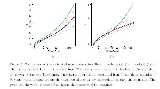
First, considering the threshold model for known covariates S with the corresponding the density function h(s). The return level \(z_T\),i.e. the T- year return, is obtained by solving the equation $$\exp \left \{ - \displaystyle \int_{-\infty}^{\infty} \left[1 + \xi(s) \left( \frac{z_T-\mu(s)}{\sigma(s)}\right) \right]^{-1/\xi(s)} h(s) ds \right\} = 1 - \frac{1}{T}. $$ which integrates over covariate space where \(\mu(s), \sigma(s), \xi(s)\) are GEV parameters incorporating the scalar covariates when S=s. Generally, the return level solution can be solved by numerical optimisation algorithm since it does not have an analytical form.
Note that there are many way to incorporate the covariates into model such as linear model with appropriate inverse-link function (David and Smith (1990)) or generalise addictive models (Yee and Stephenson, 2007) or splines ( Pauli and Coles, 2001).
However, it not usually the case that covariates are observed, hence we need to take into account for unknown covariates, namely random effects into the model. Random effects are used to account for unexpected behaviour in extreme value applications and therefore, can be include in different way into all three parameters of the point process. Here Ross Towe et al. made the assumption that these random effects stay the same within each years and independent and identically distributed over years, whose joint distribution follow the multivariate Normal distribution with zero mean and covariance matrix including the unit deviation for each random effects and their mutual correlations.
Unlike the observed covariate case, obtaining maximum likelihood estimators for parameters and random effects is very hard, however, can be solved effectively by the Bayesian methods and adaptive MCMC algorithms (method of Eastoe (2018)). Despite of the convenient use of this method, it is useful to spots-check the trace plots to assess the convergence, mixing, burn-in of the chains.
Similar for the known covariate case, a single cross-year return level estimates can be obtained by solving the equations involving the integral over random effects, but there is a closed-form for the return level within one block.
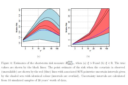
Then a short-term risk measure is proposed which use to size of the largest event up to this point in the block to predict for whether there is a higher/lower/same risk for the rest of a block, i.e. suppose that at time t within the block we observe a T-year event of size \(z_T\) and we want to determine for the remainder of block, the probability of observing an event, whose size is greater than \(z_T\) . For both observed and unknown covariates, the variance of this new measure are given in a closed form expressions.