Changing Extremes
21st February 2016
The MRes students of STOR-i are currently in the middle of our short research topic projects. These involve writing a
literature review into one of the topics presented to us a few weeks ago. Some of these were discussed in
Optimising with Ants and Ice-cream Cones,
Can Hamiltonian Win At Monte Carlo? and Gaussian Processes.
The topic I have chosen to look at in more detail is an extension of the subject of
Tails, Droughts and Extremes, that is Non-stationary Extremes. This was presented by
Dr. Emma Eastoe as part of the Extreme Value Research Topic. A
conversation with her about potential directions for me to go into resulted with quite a long list of papers for me to
read about the subject, and a wealth of different approaches dependent on how one wishes to attack the problem.
The main problem with using standard extreme value theory to model many problems, such as data coming from a time series,
is that we implicitly assume that the data are independent and come from a stationary distribution. However, as
Chavez-Demoulin and Davison put it in their review of the subject in 2012:
"Stationary time series rarely arise in applications, where seasonality, trend, regime changes and dependence on external
factors are the rule rather than the exception, and this must be taken into account when modelling extremes."
Non-stationary extreme value theory is an attempt to model such behaviour. From my reading, I have found a number of
methods that seem to fall into three main categories:
- Allowing model parameters (from Generalised Extreme Value (GEV) distribution or Generalised Pareto (GP) distribution) to follow a Dynamic Linear Model (DLM)
- Allowing model parameters to vary with covariates such as time, either as a deterministic model or by splitting data into blocks
- Using the entire data set (not just the extremes) to find the non-stationary behaviour, then removing to allow treatment of extremes as stationary (pre-processing)
The first of these uses a GEV distribution, whereas the second two tend to be based around a Poisson Process
of exceedances of a threshold $u$ or the GP distribution. Each of these methods have positive points and draw
backs. In this post, I would like to discuss each very briefly as I understand them.
DLM
A DLM allows the model parameters to evolve with a random element. A state vector at time $t$, $\theta_t$, of
various characteristics of the system is chosen. This evolves using a matrix, $G_t$, and a random vector, $\omega_t$,
from a multivariate normal distribution with covariance matrix $W$. The parameter $\alpha_t$, then depends on
$\theta_t$, another vector $F_t$ known as the regressor and a normally distributed noise term, $\epsilon_t$, with
variance $V$. A DLM is defined by $F_t,V,G_t$ and $W$. To sum up,
$$\alpha_t = F_t^T\theta_t + \epsilon_t$$
where
$$\theta_t = G_t\theta_{t-1} + \omega_t.$$
Each part can be estimated using Bayesian statistics. This was applied by
Huerta and Sanso to ozone data, where the
location parameter of a GEV was assumed to follow a DLM. They showed that this approach is that any trend, whether
short or long term, can be picked out without assuming a parametric form, making it very flexible. However, there
are many parameters to estimate which may involve a lot of computational time.
Varying Extreme Parameters with Covariates
This is by far the most common method I have come across, and there are multiple ways of going about it. Unlike the
DLM approach, it is more common to use a GP distribution, in which case the choice of $u$ is key. One way is to
split the data into predefined "seasons" that are assumed approximately stationary and then select $u$ such that
the exceedance probability, $p$, is constant. If there are more covariates involved than just time, one could allow $u$ to
vary with the covariates. This was used by
Northop and Jonathan on hurricane data. First they used Likelihood Inference to produce good regression models
for the GP parameters. From this, quantile regression is used to ensure $u$ produces the correct exceedance rate. This
idea has the difficulty of combining the uncertainty of the model of $u$ and the other parameters. It can also be quite
complicated.
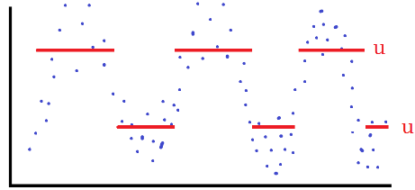
When using a GP model, the choice of threshold $u$ is crucial.
Alternatively, one could assume an underlying model, such as a sinusoidal variation, for $u$ and using the data to
choose the constants such that $p$ is roughly equal at each point of time. This model is simpler and less sophisticated
than the previous one and can be very sensitive to the model specified, so one must have a really good reason to believe
it is correct. However, it is simpler and so easier to use.
Pre-processing
The problem with the above method, particularly when covariates are involved, is that so-called "threshold stability"
of the GP distribution does not hold. That is, just because the model works for a threshold $u$, it may not work for
a threshold $v>u$. This is due to the fact that the scale and shape parameters may not use the same covariates. The
Pre-processing method uses all the data, not just the extremes, to estimate the non-stationary behaviour of the
process $Y_t$. This can then be removed to produce a new process $Z_t$. If there is a pre-existing theoretical model,
this can be used. If not,
Eastoe and Tawn suggest a
Box-Cox method of the form
$$\frac{Y_t^{\lambda_t}-1}{\lambda_t} = \mu_t + \sigma_tZ_t.$$
Once $Z_t$ has been obtained, the extremes of $Z_t$ can be analysed in a more straight forward manner. The benefits
of this approach are that the non-stationary behaviour can be estimated much more reliably than in the previous
methods. In addition, it has more statistical efficiency. On the down side, if the extremes of $Y_t$ do not follow
the same non-stationarity as the body, then $Z_t$ will require another non-stationary method. The other negative
is that it is much more complicated than the methods above.
All of these methods are interesting, and have been very interesting to read about. There does seem to be a lot of
disagreement as to which method is best, but I imagine that it is which method is the best depends very much on the
situation and application.
References
[1] Modelling time series extremes
Chavez-Demoulin V., Davison A. C., REVSTAT – Statistical Journal, Volume 10, Number 1, pp.109–133
(2012).
[2] Time-varying models for extreme values
Gabriel Huerta, Bruno Sanso, Environ Ecol Stat, 14, pp.285–299
(2007).
[3] Threshold modelling of spatially dependent
non-stationary extremes with application to hurricane-induced wave heights
P. J. Northrop and P. Jonathan, Environmetrics, Vol.22(7), pp.799-809
(2011).
[4] Modelling non-stationary
extremes with application to surface level ozone E. F. Eastoe and J. A. Tawn, JRSS, Appl. Statist. 58, Part 1,
pp. 25–45 (2009).