1.2 Conjugacy

(Binomial sample.) Suppose our likelihood model is $x\sim \text{Binomial }(n,\theta )$, and we wish to make inferences about $\theta$, from a single observation $x$.

So

$$f(x|\theta )=\left(\genfrac{}{}{0pt}{}{n}{x}\right){\theta }^x{(1-\theta )}^{n-x};$$

So, in this case, suppose we can represent our prior beliefs about $\theta$ by a beta distribution:

$$\theta \sim \text{Beta }(p,q)$$

so that

	$\pi (\theta )$	$=$	${\displaystyle \frac{\mathrm{\Gamma }(p+q)}{\mathrm{\Gamma }(p)\mathrm{\Gamma }(q)}}{\theta }^{p-1}{(1-\theta )}^{q-1}\mathit{\hspace{1em}\hspace{0.5em}\hspace{1em}}(0\le \theta \le 1)$
		$\propto$	${\theta }^{p-1}{(1-\theta )}^{q-1}.$

The parameters of this distribution are $p>0$ an d $q>0$. (They are NOT probabilities and may have any positive value.) The mean and variance of this distribution are

	$\mathrm{E}(\theta )$	$=m={\displaystyle \frac{p}{p+q}}$
	$\text{and}\mathrm{Var}(\theta )$	$=v={\displaystyle \frac{pq}{{(p+q)}^2(p+q+1)}}.$

The Beta distribution is written as

$\pi (\theta )$

$=$

${\displaystyle \frac{{\theta }^{p-1}{(1-\theta )}^{q-1}}{\text{B}(p,q)}}\text{where}\text{B}(p,q)={\displaystyle \frac{\mathrm{\Gamma }(p)\mathrm{\Gamma }(q)}{\mathrm{\Gamma }(p+q)}}={\displaystyle {\int }_0^1}{\theta }^{p-1}{(1-\theta )}^{q-1}\text{d}\theta .$

We call $\text{B}(p,q)$ the beta function; don’t confuse it with the distribution.

In Figure Figure 1.10 (Link) some simple cases of the beta distribution are shown.

Bayes Rule Now we apply Bayes Theorem using this prior distribution:

	$\pi (\theta \mid x)$	$\propto$	$\pi (\theta )f(x|\theta )$
		$\propto$	${\theta }^{p-1}{(1-\theta )}^{q-1}\times {\theta }^x{(1-\theta )}^{n-x}$
		$=$	${\theta }^{p+x-1}{(1-\theta )}^{q+n-x-1}$
		$=$	${\theta }^{P-1}{(1-\theta )}^{Q-1}$

There is only one density function proportional to this, so it must be the case that

$$\theta |x\sim \text{Beta }(P,Q).$$

The updates are

	$P$	$\leftarrow p+x$
	$Q$	$\leftarrow q+n-x.$		(Updates for Beta prior with a Binomial likelihood)

In other words, the number of successes to added to the first parameter of the Beta and the number of failures to the second parameter. This does not have to be done all at once. It can be done observation by observation.

Sequential updating of belief in a parameter

.

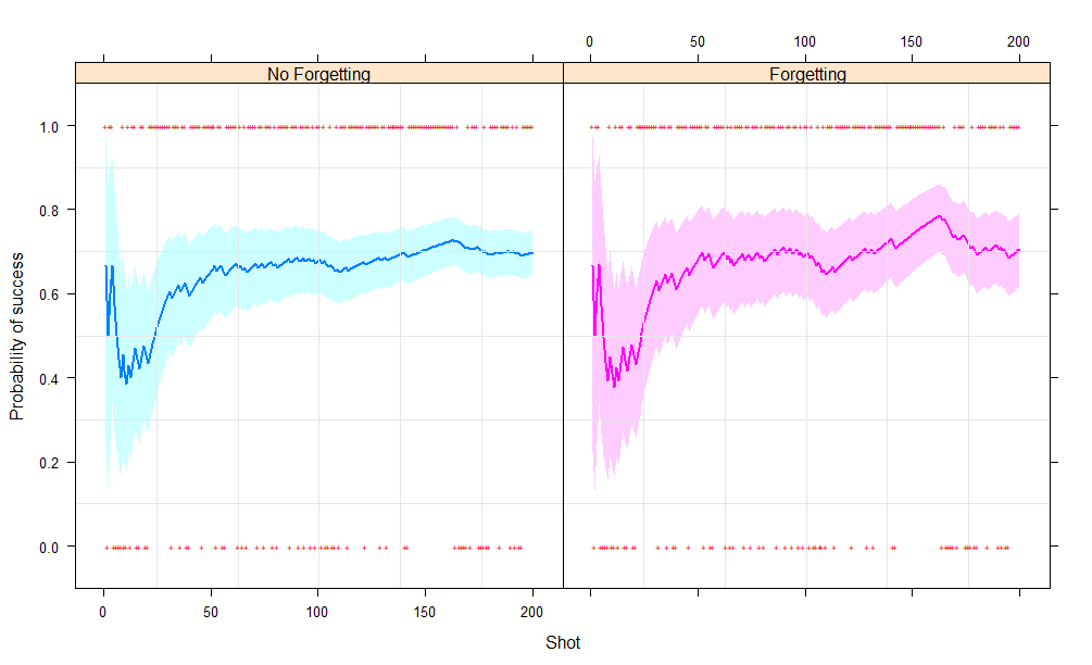
If the data consists of a sequence of shots on goals by a player. They are denoted by $Y=1,1,0,1.$ Then our belief in the ability of the player can be updated sequentially.

$\text{Beta }(1,1)\stackrel{y=1}{\to }\text{Beta }(2,1)\stackrel{y=1}{\to }\text{Beta }(3,1)\stackrel{y=0}{\to },\text{Beta }(3,2)\stackrel{y=1}{\to }\text{Beta }(4,2)$

The expected sucess rates are

${\widehat{\pi }}_0={\displaystyle \frac{1}{2}},{\widehat{\pi }}_1={\displaystyle \frac{2}{3}}{\widehat{\pi }}_2={\displaystyle \frac{3}{4}},{\widehat{\pi }}_3={\displaystyle \frac{3}{5}},{\widehat{\pi }}_4={\displaystyle \frac{4}{6}}$

Let us take an example of a run of successes and failures in a basketball game. For each success $p\to p+1$. For each failure $q\to q+1$

y <- c(1, 0, 1, 1, 0, 0, 0, 0, 1, 0, 0, 1, 0, 1, 1, 0, 0, 1, 1, 0, 0, 1,
    1, 1, 1, 1, 1, 1, 1, 1, 1, 0, 1, 1, 1, 0, 1, 1, 0, 0, 1, 1, 1, 1, 1,
    1, 1, 1, 0, 1, 1, 0, 1, 1, 1, 0, 1, 0, 1, 1, 1, 1, 1, 0, 1, 1, 1, 0)
ΨΨ#several rows ommitted
p <- 1 ;q <- 1
mean <- rep(0, 200); uq <- rep(0, 200); lq <- rep(0, 200)
for (i in 1:200) {
    p <- p + y[i]
    q <- q + 1 - y[i]
    mean[i] <- p/(p + q)
    lq[i] <- qbeta(0.025, p, q)
    uq[i] <- qbeta(0.975, p, q)
}

In stationary models (when $\theta$ is fixed) as more and more observations are made we become more and more certain about the parameter an intervals for the parameter ($\theta$) become narrower.

In a model with forgetting, the parameter $\theta$ changes with time. A good example of this is when $\theta$ is the current form of a current sports team. As the team changes $\theta$ the form of the team changes. When $\theta$ changes recent results are judged more relevant than the results of games from the distant past.

Click this link for a good video on Bayesian inference on a beta distribution: https://www.coursera.org/learn/bayesian/lecture/xFRKb/inference-on-a-binomial-proportion ‘

Suppose we have a random sample (i.e. independent observations) of size $n$, $x=(x_1,x_2,\mathrm{\dots },x_n)$ of a random variable $X$ whose distribution is Poisson $\left(\theta \right)$ Then

	$f(x|\theta )$	$=$	${\displaystyle \prod _{i=1}^n}{\displaystyle \frac{e^{-\theta }{\theta }^{x_i}}{x_i!}}=L(\theta ;x)$
		$\propto$	$e^{-n\theta }{\theta }^{\mathrm{\Sigma }{x}_i}$

As in the binomial example, prior beliefs about $\theta$ will vary from problem to problem, but we’ll look for a form which gives a range of different possibilities, but is also mathematically tractable.

case we suppose our prior beliefs can be represented by a gamma distribution:

$$\theta \sim \text{Gamma }(p,q),$$

so

$$\pi (\theta )=\frac{q^p}{\mathrm{\Gamma }(p)}{\theta }^{p-1}\exp \{-q\theta \}\mathit{\hspace{1em}\hspace{0.25em}}(\theta >0).$$

The parameter $p>0$ is a shape parameter, and $q>0$ is a scale parameter. The mean and variance of this distribution are

$$\text{E }(\theta )=m=\frac{p}{q}\text{and}\mathrm{Var}(\theta )=\mathrm{v}=\frac{\mathrm{p}}{{\mathrm{q}}^2}.$$

Assume we have a Poisson likelihood with a gamma prior then by applying Bayes’ Theorem with this prior distribution we get,

	$\pi (\theta \mid x)$	$\propto$	${\displaystyle \frac{q^p}{\mathrm{\Gamma }(p)}}{\theta }^{p-1}\exp \{-q\theta \}\times \exp \{-n\theta \}{\theta }^{\mathrm{\Sigma }{x}_i}$
		$\propto$	${\theta }^{(p+\mathrm{\Sigma }{x}_i-1)}\exp \{-(q+n)\theta \}$
		$=$	${\theta }^{P-1}\exp (-Q\theta ).$

Again, there is only one density function proportional to this, so it must be the case that

$$\theta |x\sim \text{Gamma }(P,Q),$$

This is nother gamma distribution whose parameters are modified by the sum of the data, ${\sum }_{i=1}^n{x}_i$, and the sample size $n$. The updates are

	$P$	$\leftarrow p+{\displaystyle \sum _{i=1}^n}{x}_i$
	$Q$	$\leftarrow q+n.$		(Updates for Gamma prior with a Poisson likelihood)

A nice video example on Poisson-Gamma conjugacy: https://www.coursera.org/learn/bayesian-statistics/lecture/tR5ne/lesson-8-1-poisson-data

Let us take an example of drug arrest from a particular patrol car and update our parameters sequentially: $p\to p+y$ and $q\to q+1$.

y <- c(0, 1, 0, 0, 7, 0, 0, 0, 0, 0, 1, 3, 0, 4, 0, 1, 0, 2, 2, 0, 0, 0,
    0, 0, 0, 0, 0, 2, 0, 0, 0, 3, 1, 0, 0, 1, 0, 0, 0, 0, 2, 1, 0, 1, 0,
    0, 0, 0, 0, 0, 0, 1, 0, 1, 0, 3, 0, 0, 0, 2, 0, 0, 4, 0, 0, 0, 0, 0,
    0, 1, 0, 0, 0, 0, 1, 0, 0, 1, 1, 0, 0, 0, 0, 0, 0, 0, 0, 0, 0, 0, 0,
    3, 0, 0, 1, 0, 0, 0, 1, 0, 0, 0, 0, 0, 0, 0, 0, 0, 0, 2, 1, 2, 1, 0,
    0, 0, 1, 2, 1, 2, 11, 2, 4, 0, 2, 4, 7, 5, 12, 6, 4, 6, 0, 4, 9, 4,
    8, 7, 2, 9, 10, 16, 19, 2)
p <- 1; q <- 1;n <- length(y)
mean <- rep(0, n); luq <- rep(0, n);lq <- rep(0, n)
for (i in 1:n) {
    p <- p + y[i];   q <- q + 1;   mean[i] <- p/q
    lq[i] <- qgamma(0.025, p, q);  uq[i] <- qgamma(0.975, p, q)
}

The panel on the left shows drug related reports, The posteriors are calculated sequentially. Here all observations are considered equally. Note how the uncertainty expected number of drug arrests (the shaded region) goes down in time. In the second panel the past is downweighted and recent history is emphasised.

Let $i\in \{1,2,\mathrm{\dots },20\}$ denote the home team and $j\in \{1,2,\mathrm{\dots },20\}$ denote the away team and the games in chronological labelled as $t=1,\mathrm{\dots },380$.

	$x_{i,j}^t$	$\sim \text{Poisson }\left({\mu }_{i,j}\right),$	${\mu }_{i,j}={\alpha }_i{\beta }_j\gamma$		(Likelihood for goals of home team )
	$y_{j,i}^t$	$\sim \text{Poisson }\left({\lambda }_{j,i}\right),$	${\lambda }_{j,i}={\alpha }_j{\beta }_i.$		(Likelihood for goals of away team)

where ${\alpha }_i$ denotes the attacking strength of team $i$, ${\beta }_j$ is the defensive strength of team $j$ and $\gamma$ is the common home ground advantage. The priors for the Poisson model are given below. $\delta$ is fixed at say $\delta =10$.

	${\alpha }_i$	$\sim \text{Gamma }(\delta ,\delta )$		(Priors for attacking strengths)
	${\beta }_j$	$\sim \text{Gamma }(\delta ,\delta )$		(Priors for defensive strengths)
	$\gamma$	$\sim \text{Gamma }(\delta ,\delta )$		(Priors for home ground advantage)

Let us say Liverpool is playing Arsenal at Home. The prior attacking and defensive strengths before the game are

	${\alpha }_L$	$\sim \text{Gamma }(2,1)$	${\alpha }_A\sim \text{Gamma }(3,2)$
	${\beta }_L$	$\sim \text{Gamma }(1,3)$	${\beta }_A\sim \text{Gamma }(3,4)$
	$\gamma$	$\sim \text{Gamma }(3,2)$

Let us say Liverpool win 4-1.

1. 1.

   Find the expected attacking strength, defensive strengths and HGA before the game.

2. 2.

   Find the prior expected score.

3. 3.

   Write out the likelihood for the scores of the home and away teams.

4. 4.

   Find the posterior distributions of all five parameters.

5. 5.

   Update the Gamma parameters for their attacking and defensive strengths, and HGA after game.

6. 6.

   Which teams improved their attacking strength and defensive strengths?

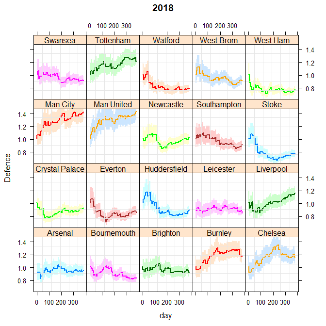
Attacking strength shown through the 2017-18 football league season. All goals are modelled as Poisson. All teams start with the same prior (ie the same ability). The shaded region shows the region between the upper and lower quartiles.

The following is a useful result for identifying normal distributions. If $\mu$ is a parameter with probability density function $f(\mu )$ satisfying

$$f(\mu )\propto \exp \left(-\frac{1}{2}\{A{\mu }^2-2B\mu \}\right),$$

iff $\mu \sim \text{Normal }(B/A,1/A).$
PROOF $(⟸)$

	$\mu$	$\sim \text{Normal }(B/A,1/A)$
	$⟹-2\log (f(\mu ))$	$=A{\left(\mu -{\displaystyle \frac{B}{A}}\right)}^2$
		$=A{\mu }^2-2B\mu +{\displaystyle \frac{B^2}{A}}$
	$⟹f(\mu )$	$\propto \exp \left(-{\displaystyle \frac{1}{2}}\{A{\mu }^2-2B\mu \}\right)$

We now pair up the likelihood with a prior for $\mu$.

	$Y_i$	$\sim \text{Normal }(\mu ,\frac{1}{\tau }),i=1,2,\mathrm{\dots },n$		(The likelihood)
	$\mu$	$\sim \text{Normal }({\mu }_0,\frac{1}{{\tau }_0})$		(The prior)

We now show that the conjugate prior for the mean of the normal using the result above

	$\pi (\mu |\text{𝐲})$	$\propto L(\mu ;y_i)\pi (\mu )$
		$\propto \exp \left(-{\displaystyle \frac{\tau }{2}}{\displaystyle \sum _{i=1}^n}{(y_i-\mu )}^2\right)\exp \left(-{\displaystyle \frac{{\tau }_0}{2}}{(\mu -{\mu }_0)}^2\right)$
		$\propto \exp \left(-{\displaystyle \frac{\tau }{2}}(n{\mu }^2-2\mu {\displaystyle \sum _{i=1}^n}{y}_i)\right)\exp \left(-{\displaystyle \frac{{\tau }_0}{2}}({\mu }^2-2\mu {\mu }_0)\right)$
		$\propto \exp \left(-{\displaystyle \frac{n\tau +{\tau }_0}{2}}{\mu }^2-\mu (n\tau \overline{y}+{\tau }_0{\mu }_0)\right)$
		$\propto \exp -{\displaystyle \frac{n\tau +{\tau }_0}{2}}{\left(\mu -{\displaystyle \frac{\tau n\overline{y}+{\tau }_0{\mu }_0}{n\tau +{\tau }_0}}\right)}^2$
	$⟹\mu \mid y,\tau$	$\sim \text{Normal }(\frac{\tau n\overline{y}+{\tau }_0{\mu }_0}{n\tau +{\tau }_0},\frac{1}{n\tau +{\tau }_0})$		(1.1)

1. Prior precision = ${\tau }_0$.

2. Sample precision = $n\tau$.

3. Posterior Precision ${\tau }_p\leftarrow {\tau }_0+n\tau$.

4. Posterior precision = prior precision + sample precision

5. Prior mean = ${\mu }_0$.

6. Sample mean = $\overline{y}$.

7. Posterior mean ${\mu }_p\leftarrow \frac{n\tau \overline{y}+{\tau }_0{\mu }_0}{n\tau +{\tau }_0}$

8. =${\gamma }_0{\mu }_0+{\gamma }_s\overline{y}$.

9. ${\gamma }_0=\frac{{\tau }_0}{n\tau +{\tau }_0}=\frac{\frac{{\tau }_0}{\tau }}{n+\frac{{\tau }_0}{\tau }}$

10. ${\gamma }_s=\frac{n\tau }{n\tau +{\tau }_0}=\frac{n}{n+\frac{{\tau }_0}{\tau }}$

11. Posterior mean = weighted sum of the prior mean and the sample mean

12. ESS of a Gaussian prior with respect to a Gaussian sample $\frac{{\tau }_0}{\tau }$.

Observations to be made A number of observations can be made:

1. (1)

   Note that the effective sample size $n_0=\frac{{\tau }_0}{\tau }$ or ${\tau }_0=n_0\tau$.

2. (2)

   Observe that ‘posterior precision’ = ‘prior precision’ + $n\times$ ‘precision of each data item’.

3. (3)

   As $n\to \mathrm{\infty }$, then (loosely)

   $$\mu |y\sim \text{Normal }(\overline{y},\frac{{\sigma }^2}{n})$$

   so that the prior has no effect in the limit.

4. (4)

   As uncertainty contained in the prior increases or ${\sigma }_0^2\to \mathrm{\infty }$, or equivalently the prior precision decreases or ${\tau }_0\to 0$, we again obtain

   $$\mu |y\sim \text{Normal }(\overline{y},\frac{{\sigma }^2}{n})$$

5. (5)

   Note that the posterior distribution depends on the data only through $\overline{y}$ and not through the individual values of the $y_i$ themselves. Again, we say that $\overline{y}$ is sufficient for $\mu$.

Let us take an example data set :Yearly suicides in Australia per 100000 individuals. We update the mean one observation at a time. Bayes theorem gets applied at each time step $i=1,2,\mathrm{\dots }$ using the previous mean, ${\mu }_{i-1}$, in the prior for the current mean ${\mu }_i$.

	${\mu }_i$	$\sim \text{Normal }({\mu }_{i-1},\frac{1}{{\tau }_{i-1}})$		(The   Prior )
	$y_i$	$\sim \text{Normal }({\mu }_i,\frac{1}{\tau })$		(The   Likelihood )
	${\mu }_i\mid y_i$	$\sim \text{Normal }(\frac{{\mu }_{i-1}{\tau }_{i-1}+y_i\tau }{{\tau }_{i-1}+\tau },\frac{1}{{\tau }_{i-1}+\tau })$		(The   Posterior)
		$\sim \text{Normal }({\mu }_{i-1}+\underset{\mathrm{Gain}}{\underbrace{\left(\frac{\tau }{\tau +{\tau }_{i-1}}\right)}}\underset{\mathrm{error}}{\underbrace{(y_i-{\mu }_{i-1})}},\frac{1}{\tau +{\tau }_{i-1}})$

Let

	$Y\mid \tau$	$\sim \text{Normal }(\mu ,\frac{1}{\tau })$
	$f(y\mid \tau )$	$\propto {\tau }^{\frac{n}{2}}{e}^{-{\sum }_{i=1}^N{(y_i-\mu )}^2\tau /2}$

Since $\mu$ is fixed then $S={\sum }_{i=1}^N{(y_i-\mu )}^2$ will also be fixed. Thus the prior is $\tau \sim \text{Gamma }(p,q)$.

	$\pi (\tau )$	$\propto {\tau }^{p-1}{e}^{-q\tau }.$		(The prior)
	$f(y|\tau )$	$\propto {\tau }^{\frac{n}{2}}{e}^{-S\tau /2}.$		(The likelihood)
	$\pi (\tau |y,\mu )$	$\propto \pi (\tau )f(y|\tau )$
		$\propto {\tau }^{p+\frac{n}{2}-1}{e}^{-\tau \left(\frac{S}{2}+q\right)}$
	$⟹\tau \mid y,\mu$	$\sim \text{Gamma }(\frac{n}{2}+p,\frac{{\sum }_{i=1}^n{(y_i-\mu )}^2}{2}+q).$		(The posterior)

The normal distribution (mean, $\mu$, known) So the updates for the parameters of the Gamma distribution are

	$P$	$\leftarrow p+{\displaystyle \frac{n}{2}}$
	$Q$	$\leftarrow q+{\displaystyle \frac{{\sum }_{i=1}^n{(y_i-\mu )}^2}{2}}$		(Updates for Gamma prior with a normal likelihood)

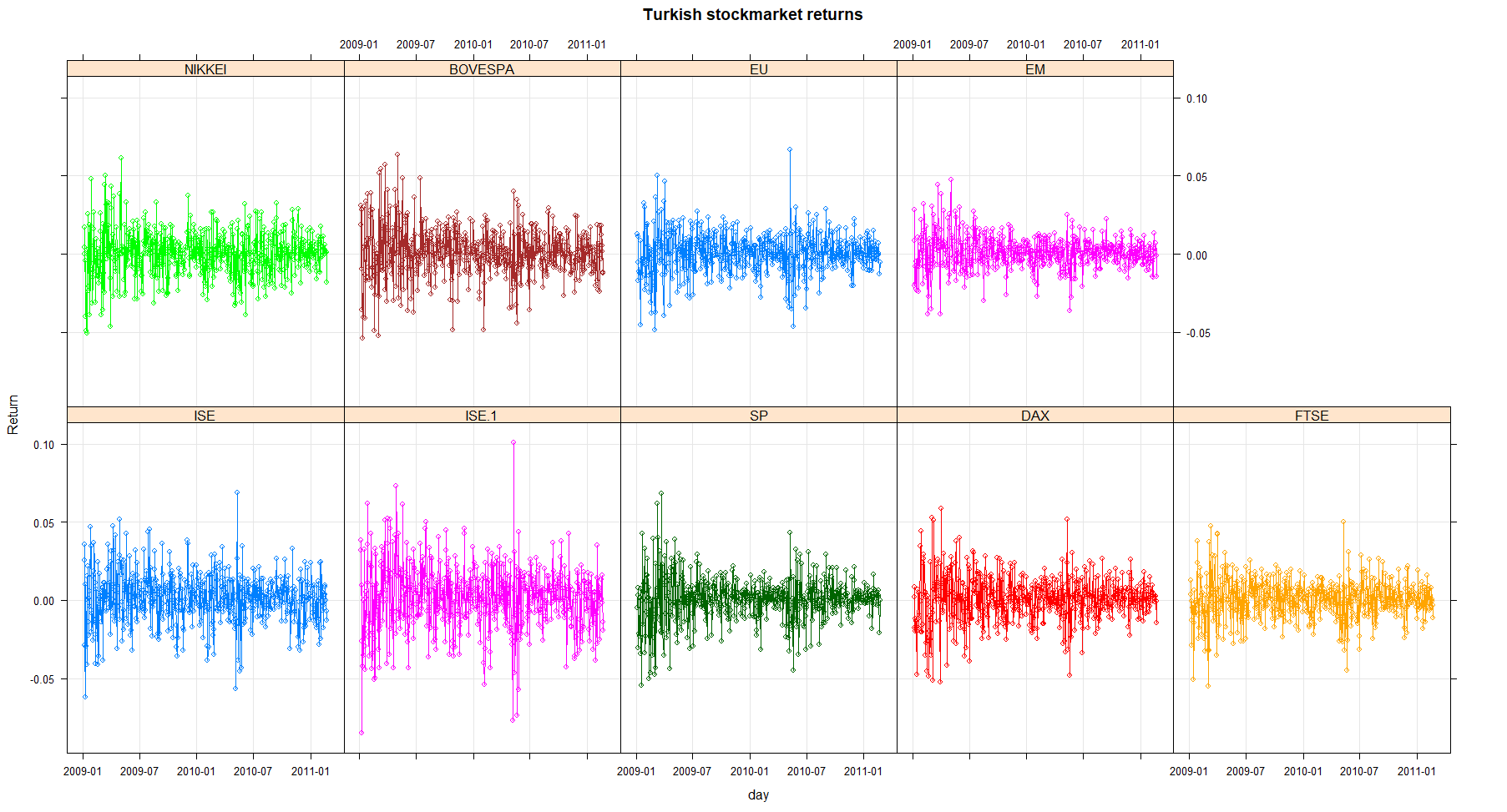
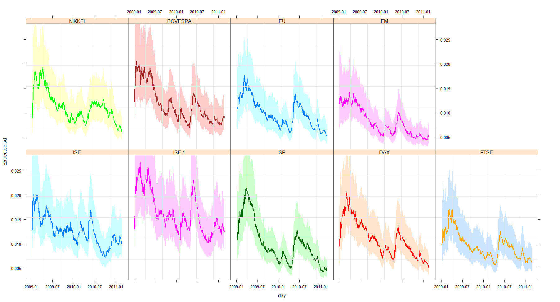
The Laplacian distribution is useful for modeling distributions with heavy tails such as those found in stock-market returns. We model the returns as

$$y_i\mid \mu ,\tau \sim \text{Laplace }(\mu ,\frac{1}{\tau })$$

where has a density given by

$$f(y_i|\tau ,\mu )=\tau \exp (-\tau \left|y_i-\mu \right|),i=1,2,\mathrm{\dots },n.$$

where $\tau$ is not the precision. The Laplacian has a variance given by $\text{Var }(y_i\mid \mu ,\tau )=2{\tau }^{-2}$. In volatility modelling we are interested in how the variance of observations change (not the mean). We set the mean of the Laplacian to zero.

$$f(y|\tau )\propto {\tau }^n{e}^{-\tau {\sum }_{i=1}^n|y_i|}.$$

When the prior is given as $\tau \sim \text{Gamma }(p,q)$, The posterior becomes

	$\pi (\tau |y)$	$\propto \pi (\tau )f(y|\tau )$
	$⟹\tau \mid y$	$\sim \text{Gamma }(n+p,{\sum }_{i=1}^n|y_i|+q).$

So the updates for the Gamma distribution are

	$P$	$\leftarrow p+n$
	$Q$	$\leftarrow q+{\displaystyle \sum _{i=1}^n}|y_i|.$		(Updates for Gamma prior with a Laplacian likelihood)

Lehman Brothers filed for bankruptcy on 15 September 2008, prompting a fall in the FTSE 100 of 4%. It was the beginning of a slump that by Christmas of that year had resulted in 23.4% being wiped off the value of Britain’s top 100 companies.

In a matter of minutes (May 2010) the Dow Jones index lost almost 9% of its value in a sequences of events that quickly became known as ”flash crash”. Hundreds of billions of dollars were wiped off the share prices of household name companies. But the carnage, which took place at a speed never before witnessed, did not last long. The market rapidly regained its composure and eventually closed 3% lower. In just 20 minutes, 2 Bn shares worth $56 Bn had changed hands.

A dataset that illustrates these shocks is shown here

Let $X_1,\mathrm{\dots }{X}_n$ be independent variables having the Gamma $(k,\theta )$ distribution, where $k$ is known.

$$L(\theta ;x)\propto {\theta }^{nk}\exp \{-\theta \mathrm{\Sigma }{x}_i\}.$$

Now, studying this form, regarded as a function of $\theta$ suggests we could take a prior of the form

$$\pi (\theta )\propto {\theta }^{p-1}\exp \{-q\theta \}$$

that is, $\theta \sim \text{Gamma }(p,q)$, since then by Bayes’ Theorem

$$\pi (\theta \mid x)\propto {\theta }^{p+nk-1}\exp \{-(q+\mathrm{\Sigma }{x}_i)\theta \},$$

and so $\theta |x\sim \text{Gamma }(p+nk,q+\sum x_i)$. So the updates for the Gamma distribution are

	$P$	$\leftarrow p+nk$
	$Q$	$\leftarrow q+{\displaystyle \sum x_i}$		(Updates for Gamma prior with a Gamma likelihood)