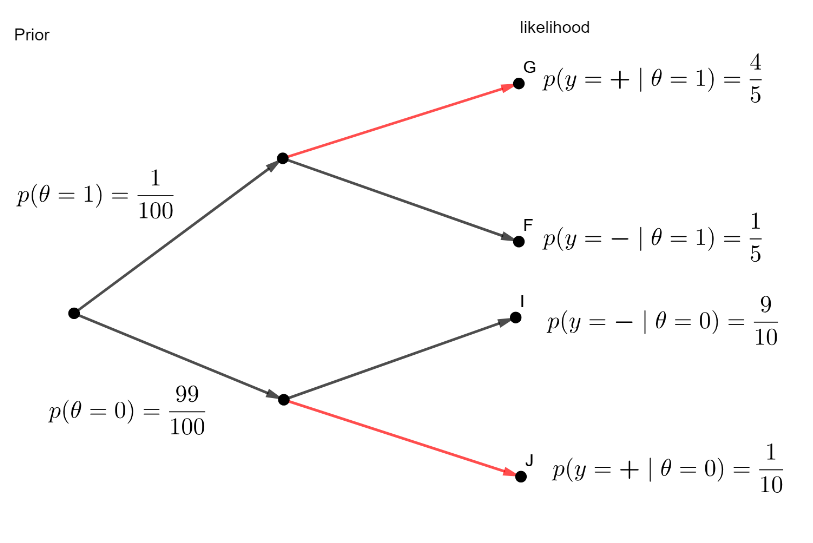
1% of women have breast cancer
80% of mammograms detect breast cancer when it is there
10% of mammograms detect breast cancer when itâs not there
Given that a patient tests positive, what is the probability she has breast cancer?
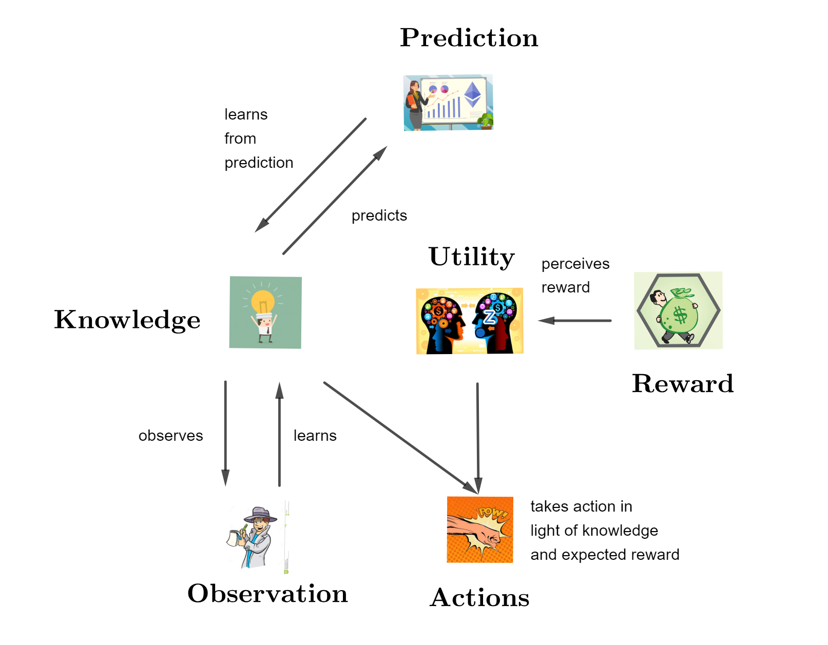
The essence of the Bayesian approach is to treat the unknown parameter as a random variable, specify a prior distribution for representing your beliefs about prior to having seen the data, use Bayes’ Theorem to update prior beliefs into posterior probabilities, and draw appropriate inferences.
Statistics is the study of reasoning in the presence of uncertainty.
Uncertainty should be measured only by conditional probability.
A probability distribution shows information. The amount of information is proportional to the precision or the reciprocal of the variance.
Data uncertainty is so measured, conditional on the parameters (through the likelihood function).
It is only by using probability that we can achieve coherence (logically connected or consistent).
Rational belief (or knowledge) is updated upon fresh observations using Bayes’ theorem.
Bayesian and classical statisticians deal with the following statistical concepts and problems in fundamentally different ways.
What is probability?
What is fixed and what is random?
The nature of uncertainty
How uncertainty is expressed
What an interval means?
How to deal with nuisance parameters?
How prior scientific knowledge is made use of?
How expected utility or loss is calculated
For each numerical value , our prior distribution describes our belief in .
For each our sampling model describes our belief that would be the outcome of our study if we knew to be true.
Once we obtain the data , the last step is to update our beliefs about . For each numerical value of , our posterior distribution describes our updated belief that is the true value, having observed data set . This is obtained via Bayes rule:
is called the marginal likelihood and depicts the evidence in favour of the model being considered and is given by, when is continuous, by .
Because the marginal likelihood does not involve , Bayes theorem is often written as
In the middle of the last century several brilliant statisticians struggled to formalise or create a clear set of fundamental rules for inductive (or statistical) thinking. There were two main groups with contrasting philosophies : the classical school and the Bayesian school. However even within each of these main groups there were disagreements and these splits still exist today. The champion of the classical school was Ronald Fisher who developed and promoted his methods prior to the second world war. These ideas quickly spread and became widely used by statistical communities. Dennis Lyndley was the champion of the Bayesian school. He was driven by a desire to make statistics a formal axiomatic and coherent system. To do this he used only the axioms of probability (formulated by Kolmorogov) and the concept utility from the work of Savage.
Ronald Fisher had a enormous impact on statistical thinking and practice with his theory of likelihood. This theory revolutionized statistical thinking at the time and methods that used it came into widespread practice. This theory, like many other theories before, had its weaknesses and did not please everybody. Fisher’s theory of hypothesis testing came under sustained attack even within the classical statistical community. Many of Fisher’s detractors argue that some of his ideas are thought to be responsible for widespread confusion and misunderstanding among scientists. The term ”statistical significance” measured by a p-value causes widespread confusion today.
Some essential elements of the Fisher’s theory are the following:
Saw probability as a long run proportion and not as degree of rational belief.
Parameters were treated as fixed but unknown. Because the parameters are fixed it made no sense to give them probability distributions.
The likelihood of a parameter was the fundamental measure of uncertainty.
Uncertainty of a parameter is related to the variability of a sample statistic (and described by Fisher’s information).
Uncertainty of a hypothesis is measured by a -value which gives a measure of strength of evidence against the null hypothesis. The p-value is defined as the probability of obtaining a test statistic at least as extreme as the one that was actually observed, assuming that the null hypothesis is true. The rejection of this idea lead to a big split among the classical statisticians and the reformulation of hypothesis testing by Neyman and Pearson as a decision problem with type-I and type II error.
Motivated by the need for an axiomatic system for statistics.
A wider definition of uncertainty than merely sampling uncertainty. All kinds of uncertainty including parameter, model uncertainty, measurent uncertainty. All of these are only be measured by probability.
Probability means degree of rational belief and is updated as new observation become available.
Probability is subjective and is conditional on the knowledge, , or experience of the individual.
https://www.youtube.com/watch?v=YsJ4W1k0hUg&index=3&list=PLFDbGp5YzjqXQ4oE4w9GVWdiokWB9gEpm
Defined an objective prior to represent ignorance or lack of any prior information.
Objective priors such as the Jeffreys’ prior have excellent frequentest properties such as good coverage.
Many statisticians from the objective school attempted to unify Bayesian and classical statistics using objective priors. These attempts have only been partially successful.
Bayesian analysis gives a more complete inference in the sense that all knowledge about , available from the prior and the data is represented in the posterior distribution. That is, is the inference. Still, it is often desirable to summarize that inference in the form of a point estimate, or an interval estimate.