SIMULATION NON-STATIONARY ARRIVAL PROCESS
16th, April, 2019.
Input themselves are generally not of interest and the outputs that the inputs imply are usually of greater interest. It is apparent that inaccurate judgement about input modelling can lead to more error. Since fitting distributions to available data using statistical framework as maximum likelihood estimation is required to understand their inference, our post will focus more on explaining how to avoid errors in input modelling in some certain cases.
Let see one example that we usually face when analysing the queueing in the hospital reception system. There is an electronic server with a touch screen replacing the human receptionist. In practical, there are some kinds of customers who are less comfortable using the electronic receptionist, then the service times for each inviduals may be more variable or slower. The aim is to evaluate the additional delay that this situations might cause. Hospital record data are available to calculate the overall arrival rate. Since customers can make independent decision when they arrive and the exponentially distributed interarrival times are available for some simulation languages, the arrival process of a large number of potential customers are usually assumed by Poisson Process. This is the input model and to fit it, the arrival rate was usually estimated by the total number of arrivals over a certain time interval over the length of this interval.
Note that this arrival process has been treated as stationary Poisson process, i.e. constant arrival rate, which is really strong assumption. There are some obvious reasons that we can reject this assumptions.
- The distribution of the data sometimes can be different from Poisson. For instance, when a reception only serves scheduled patients and a fixed number of appointments are planned each day, then the arrival process are nearly deterministic and moreover scheduled patients typically arrive not randomly, therefore not Poisson process.
- The distribution of data can be different from day to day. What happens when the arrival rate changes over time? For example, Saturdays and Sunday are usually busier than weekdays, there could be nonstationary across weeks.
In this post, we will present two algorithm to simulate the non-stationary arrival process that can overcome some limitations that we mentioned above. Examples of nonstationary arrival processes that we meet every day are the arrival of fans to football stadium, the arrivals of e-mails to a mail serve, etc. Even though we can define the joint distribution of all the arrival times, it is more natural and convenient for simulation discrete interarrival times or the times between one arrival to the next one.
The idea of methods for simulation is to transform a basic and easily controllable input process to the input process we want. In more details, in order to obtain the nonstationary arrival process, we transform the independent and identically distributed interarrival times to the arrival rate we want while retaining a measure of variability. This makes us think about renewal process, which is the basic form of random process. Let \(N(t)\) be the arrival counting process (number of arrivals by time \( t\)) of a nonstationary arrival process. We define the integrated rate function be the expected number of arrivals by time \(t\) $$ \Lambda(t) = E(N(t))$$ and the arrival rate is define by differentiating the integrated rate function with respect to \(t\), which can be differentiable $$ \lambda(t) = \frac{d}{dt} \Lambda(t)$$ And for the equilibrium renewal process, there is a relationship between them $$ \Lambda(t) = \lambda(t) t$$
In Inversion a stationary Poisson process with rate one is used as a base, which is still a random process but with a mean interarrival times of \(1\). In order to simulate the sample of interarrival times:
- Consider the time of the \(n\)-th arrival in the stationary process and evaluate this at \( \Lambda^{-1}(t) \).This is the time of arrival in the non-stationary process.
- The previous arrival time is subtracted from this new arrival time, generating the \(n\)-th interarrival time.
- This is done iteratively to simulate a non-stationary arrival process from a stationary one.
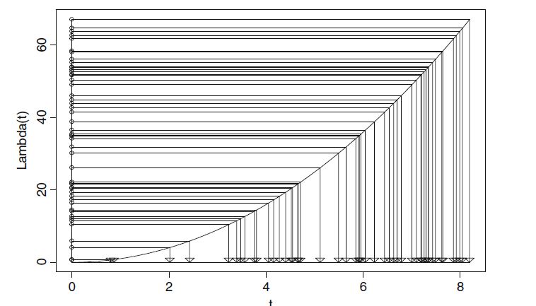
In order to see why \(\Lambda^{-1}(t)\) indeed maps the arrival times of an equilibrium renewal process with rate \(1\) into the desired nonstationary arrival process with rate \( \lambda(t)\), please find the very short proof in the references.
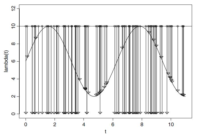
In Thinning a sample of interarrival times can be generated by:
- Let \(\tilde{\lambda} = \max_t \lambda(t)\) and generate a random number \(U \sim U(0,1)\).
- Evaluate the rate function at the time of the \(n^{\text{th}}\) arrival in the maximum rate stationary process, and then calculate the ratio \(\lambda(t)/\tilde{\lambda}\).
- If \(U \leq \lambda(t)/\tilde{\lambda}\) then we add this interarrival time, else the timer continues.
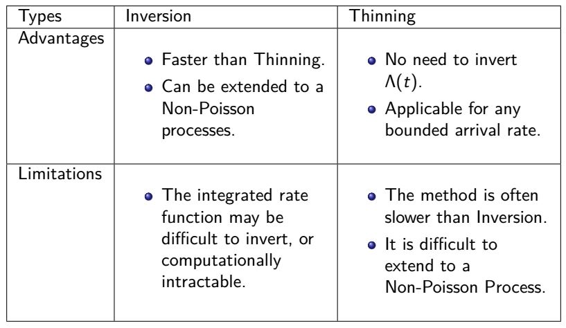
Even though both algorithm lead to arrival processes with the same desired arrival rate which changes over time, they generally do not give exactly the same processes in term of probability such as variance of the number of arrivals by time \(t\), except for the Poisson arrival process that are probabilistically the same.Here is the comparison of two algorithm by highlighting the advantage and drawback of each methods:
I hope this post can help you understand the importance of input modelling as well as how to simulate the nonstationary arrival process with the desired time-varying arrival rate.
Reference:
1. Barry Nelson, Foundations and Methods of Stochastic Simulation: A first course, 2013.