4 Bayesian statistics 331 Week 4 Multi-parameter models 4.1 The Multinomial dirichlet family 5 Week 5 Bayesian statistics: Decisions

4.2 The Normal distribution

The Normal distribution

The normal distribution is a commonly encountered distribution (because of the central limit theorem) and therefore important. Bayesian inference on the normal becomes a little more difficult because there are at least two unknowns rather than one. There are a variety of ways of carrying Bayesian inference on these two parameters and the method depends on the priors being used. Let $Y_{1},\ldots,Y_{n}$ be a set of independent variables from Let $Y_{1},\ldots,Y_{n}$ be a set of independent variables from Normal $\left({\mu},{\frac{1}{\tau}}\right)$ , where both the mean and variance are denoted by $\mu$ and $1/\tau$ respectively. Then,

\displaystyle f(y_{i}|\mu,\tau)=\frac{\tau^{1/2}}{\sqrt{2\pi}}\exp\left[-\tau% \frac{(y_{i}-\mu)^{2}}{2}\right]

(4.2)

\displaystyle f(\textbf{y}|\mu,\tau)\propto\tau^{n/2}\exp\left[-\tau\frac{\sum% _{i=1}^{n}(y_{i}-\mu)^{2}}{2}\right].

(4.3)

The Normal distribution

The two parameter exponential family

$T(y)=\begin{bmatrix}y\\ y^{2}\\ \end{bmatrix}$ and $\eta(\theta)=\begin{bmatrix}\tau\mu\\ -\tau/2\end{bmatrix}$ and therefore will have fully conjugate priors.

4.2.1 The normal distribution with improper priors

The normal distribution with improper priors

Again assuming i.i.d. Gaussian likelihood which can be expressed as

\displaystyle Y_{i}\mid\mu,\tau

\displaystyle\sim\mbox{{\rm Normal\,}$\left({\mu},{\frac{1}{\tau}}\right)$}\;% \;i=1,2,\ldots,n

Also let the sample mean sum of the squares be respectively be $\bar{y}=\frac{\sum_{i=1}^{n}y_{i}}{n}$ and $S^{2}=\sum_{i=1}^{n}(y_{i}-\bar{y})^{2}$ . The likelihood can then be expressed as

	$\displaystyle f(y_{1:n}\mid\mu,\tau)$	$\displaystyle\propto\tau^{\frac{n}{2}}\exp\left\{-\frac{\tau}{2}\sum_{i=1}^{n}% (y_{i}-\mu)^{2}\right\}$
		$\displaystyle\propto\tau^{\frac{n}{2}}\exp\left\{-\frac{\tau}{2}\sum_{i=1}^{n}% (y_{i}-\bar{y}+\bar{y}-\mu)^{2}\right\}$
		$\displaystyle\propto\tau^{\frac{n}{2}}\exp\left\{-\frac{\tau}{2}\left[\sum_{i=% 1}^{n}(y_{i}-\bar{y})^{2}+n(\bar{y}-\mu)^{2}\right]\right\}$
		$\displaystyle\propto\tau^{\frac{n-1}{2}}\exp\left\{-\frac{1}{2}S^{2}\tau\right% \}\;\tau^{\frac{1}{2}}\exp\left\{-\frac{n}{2}\tau(\mu-\bar{y})^{2}\right\}$

The normal distribution with improper priors

If we choose an improper prior of $\pi(\mu,\tau)\propto\frac{1}{\tau}$ , the joint distribution becomes

	$\displaystyle\pi(\mu,\tau\mid y)$	$\displaystyle\propto\pi(\tau,\mu)f(y_{1:n}\mid\mu,\tau)$
		$\displaystyle\propto\frac{1}{\tau}\tau^{\frac{n-1}{2}}\exp\left\{-\frac{1}{2}S% ^{2}\tau\right\}\;\tau^{\frac{1}{2}}\exp\left\{-\frac{n}{2}\tau(\mu-\bar{y})^{% 2}\right\}$
		$\displaystyle\propto\underbrace{\tau^{\frac{n-1}{2}-1}\exp\left\{-\frac{1}{2}S% ^{2}\tau\right\}}_{\mbox{{\rm Gamma\,}$\left({\frac{n-1}{2}},{\frac{S^{2}}{2}}% \right)$}}\;\underbrace{\tau^{\frac{1}{2}}\exp\left\{-\frac{n}{2}\tau(\mu-\bar% {y})^{2}\right\}}_{\mbox{{\rm Normal\,}$\left({\bar{y}},{\frac{1}{n\tau}}% \right)$}}$

The joint posterior $\pi(\mu,\tau\mid y)=\pi(\mu\mid\tau,y)\pi(\tau\mid y)$ is a product of these two distributions.

	$\displaystyle\mu\mid\tau,y$	$\displaystyle\sim\mbox{{\rm Normal\,}$\left({\bar{y}},{\frac{1}{n\tau}}\right)$}$
	$\displaystyle\tau\mid y$	$\displaystyle\sim\mbox{{\rm Gamma\,}$\left({\frac{n-1}{2}},{\frac{S^{2}}{2}}% \right)$}$		(4.4)

The marginal posterior of $\mu$

The marginal distribution of $\mu$ can be obtained by marginalisng $\tau$ from the joint distribution.

	$\displaystyle\pi(\mu\mid y)$	$\displaystyle=\int\pi(\mu,\tau\mid y)d\tau$
		$\displaystyle\propto\int\tau^{\frac{n}{2}-1}\exp\left\{-\frac{\tau}{2}\left[S^% {2}+n(\mu-\bar{y})^{2}\right]\right\}d\tau$

This is a kernel of a Gamma distribution so

	$\displaystyle\pi(\mu\mid y)$	$\displaystyle\propto\frac{\Gamma(\alpha_{p})}{\beta_{p}^{\alpha_{p}}}$
		$\displaystyle\propto\Gamma(\frac{n}{2})\left(\left[S^{2}+n(\mu-\bar{y})^{2}% \right]\right)^{-\frac{n}{2}}$

The marginal posterior of $\mu$

Finally, consider a location and scale change to $\mu$ :

t=\frac{\mu-\overline{x}}{s/\sqrt{n}}~{}~{}\mbox{where }~{}s^{2}=\frac{S^{2}}{% n-1}.

Then

	$\displaystyle\pi(t\|x)$	$\displaystyle\propto$	$\displaystyle\frac{1}{\left\{(n-1)s^{2}+(st)^{2}\right\}^{n/2}}$
		$\displaystyle\propto$	$\displaystyle\left\{1+\frac{t^{2}}{n-1}\right\}^{-n/2}.$

This is the density of a $t$ –distribution with $n-1$ degrees of freedom. That is:

t|x\sim t_{n-1}.

The distribution of a future observation (The predictive)

To find the predictive distribution $f(y_{n+1}\mid y_{1:n})$ a double integral must be carried out.

f(y_{n+1}\mid y_{1:n})=\int_{\tau}\int_{\mu\mid\tau}\pi(\mu,\tau\mid y_{1:n})f% (y_{n+1}\mid\mu,\tau)d\mu d\tau

This is easily done by carrying out these two steps

(1)

Condition on $\tau$ and integrate out $\mu$ : using

$f(y_{n+1}\mid y,\tau)=\int_{\mu\mid\tau}\pi(\mu,\tau\mid y_{1:n})f(y_{n+1}\mid% \mu,\tau)d\mu$
(2)

And then marginalisng over $\tau$ .

$f(y_{n+1}\mid y)=\int_{\tau}f(y_{n+1}\mid y,\tau)\pi(\tau\mid y)d\tau$

where $\pi(\tau\mid y)$ is given by Equation(4.4).

The distribution of a future observation (The predictive)

ntegral in (1) can be done easily using the identities for the marginal means and variances. The integral in (2) is straightforward. These integrals are not done here and are part of the coursework for this chapter. It can be shown that

y_{n+1}\mid y\sim{\rm t}_{n-1}\left(\bar{y},s^{2}\left(1+\frac{1}{n}\right)\right)

4.2.2 The fully conjugate Normal-gamma prior

Using the fully conjugate, four parameter Normal-gamma prior

\displaystyle Y_{i}\mid\mu,\tau

\displaystyle\sim\mbox{{\rm Normal\,}$\left({\mu},{\frac{1}{\tau}}\right)$}\;% \;i=1,2,\ldots,n

Also let the sample mean and variance respectively be $\bar{y}=\sum_{i=1}^{n}y_{i}$ and $s^{2}=\frac{\sum_{i=1}^{n}(y-\bar{y})^{2}}{n}$ . The likelihood can then be expressed as

	$\displaystyle f(y_{1:n}\mid\mu,\tau)$	$\displaystyle\propto\tau^{\frac{n}{2}}\exp\left\{-\frac{\tau}{2}\sum_{i=1}^{n}% (y_{i}-\mu)^{2}\right\}$
		$\displaystyle\propto\tau^{\frac{n}{2}}\exp\left\{-\frac{\tau}{2}\sum_{i=1}^{n}% (y_{i}-\bar{y})^{2}+n(\bar{y}-\mu)^{2}\right\}$
		$\displaystyle\propto\tau^{\frac{n-1}{2}}\exp\left\{-\frac{1}{2}ns^{2}\tau% \right\}\;\tau^{\frac{1}{2}}\exp\left\{-\frac{n}{2}\tau(\mu-\bar{y})^{2}\right\}$

As a function of $\mu$ and $\tau$ this is a product of a kernel of a Normal $\left({\bar{y}},{(n\tau)^{-1}}\right)$ for $\mu$ and a Gamma $\left({\frac{n+1}{2}},{\frac{ns^{2}}{2}}\right)$ for $\tau$ .

The fully conjugate, four parameter Normal-gamma prior

This parametrization of the likelihood suggests the following steps.

•

Express the priors of $\mu$ and $\tau$ as a four parameter Normal-Gamma distribution
•

Rewrite the likelihood so it has the same form.
•

By using the four parameter Normal-Gamma form of the prior.

The fully conjugate, four parameter Normal-gamma prior

We will assume $\mu$ and $\tau$ have the hierarchical conjugate priors

	$\displaystyle\tau$	$\displaystyle\sim\mbox{{\rm Gamma\,}$\left({a_{0}},{b_{0}}\right)$}$		(4.5)
	$\displaystyle\mu\mid\tau$	$\displaystyle\sim\mbox{{\rm Normal\,}$\left({\mu_{0}},{(n_{0}\tau)^{-1}}\right% )$}$		(4.6)

and will show that the conjugate posteriors using Equations (4.2.2) and (4.6) have the form

	$\displaystyle\tau\mid y$	$\displaystyle\sim\mbox{{\rm Gamma\,}$\left({a_{n}},{b_{n}}\right)$}$		(4.7)
	$\displaystyle\mu\mid\tau,y$	$\displaystyle\sim\mbox{{\rm Normal\,}$\left({\mu_{n}},{(n_{n}\tau)^{-1}}\right% )$}$		(4.8)

The fully conjugate, four parameter Normal-gamma prior

Expressions can be developed for the four parameters $\mu_{n},n_{n},a_{n},b_{n}$ . Equations (4.2.2) and (4.6) represent the Normal-Gamma family

	$\displaystyle\pi(\mu,\tau)$	$\displaystyle=\pi(\mu\mid\tau)\pi(\tau)$
		$\displaystyle\propto\tau^{a_{0}-1}\exp{\{-b_{0}\tau\}}\;\;\tau^{\frac{1}{2}}% \exp\left\{-\frac{\tau n_{0}}{2}(\mu-\mu_{0})^{2}\right\}$

By integrating over $\tau$ we can find the the marginal prior of $\mu$ $\pi(\mu)=\int_{\tau=0}^{\infty}\pi(\mu,\tau)d\tau$ and show that it has the form of the T distribution

\mu\sim\mbox{\rm t\,$\left({\mu_{0}},{\left(\frac{n_{0}a_{0}}{b_{0}}\right)^{-% 1}},{2a_{0}}\right)$}.

This leads to a posterior distribution of

\mu\mid y\sim\mbox{\rm t\,$\left({\mu_{n}},{\left(\frac{n_{n}a_{n}}{b_{n}}% \right)^{-1}},{2a_{n}}\right)$}.

The fully conjugate, four parameter Normal-gamma prior

The likelihood can be rewritten as

\displaystyle\propto\tau^{\frac{n-1}{2}}\exp\left\{-\frac{1}{2}S^{2}\tau\right% \}\;\tau^{\frac{1}{2}}\exp\left\{-\frac{n}{2}\tau(\mu-\bar{y})^{2}\right\}

This suggests a prior of the form

	$\displaystyle\pi(\mu,\tau\mid y)$	$\displaystyle=\pi(\tau\mid y)\pi(\mu\mid\tau,y)$
		$\displaystyle\propto\tau^{a_{0}-1}\exp\{-b_{0}\tau\}\;\;\tau^{\frac{1}{2}}\exp% \left\{-\frac{\tau n_{0}}{2}(\mu-\mu_{0})^{2}\right\}$

where the updates to the sufficient statistics are

$\displaystyle a_{n}$	$\displaystyle=$	$\displaystyle a_{0}+\frac{n}{2}$
$\displaystyle b_{n}$	$\displaystyle=$	$\displaystyle\frac{(n-1)s^{2}}{2}+b_{0}+\frac{1}{2}\frac{n_{0}n}{n_{0}+n}(\mu_% {0}-\bar{y})^{2}$
$\displaystyle\mu_{n}$	$\displaystyle=$	$\displaystyle\frac{n\bar{y}+n_{0}\mu_{0}}{n_{0}+n}$
$\displaystyle n_{n}$	$\displaystyle=$	$\displaystyle n_{0}+n.$

The predictive

In addition the predictive and the marginal are also available in closed from

$y^{*}\mid y\sim\mbox{\rm t\,$\left({\mu_{n}},{\frac{b_{n}(1+n_{n})}{n_{n}a_{n}% }},{2a_{n}}\right)$}$ The predictive
$y\sim\mbox{\rm t\,$\left({\mu_{0}},{\frac{b_{0}(1+n_{0})}{n_{0}a_{0}}},{2a_{0}% }\right)$}$ The marginal

Derivation of four parameter updates

	$\displaystyle f(y\mid\mu,\tau)$	$\displaystyle\propto\tau^{\frac{n-1}{2}}\exp\{-\frac{1}{2}(n-1)s^{2}\tau\}{% \tau^{\frac{1}{2}}\exp\left\{-\frac{n}{2}\tau(\mu-\bar{y})^{2}\right\}}$
	$\displaystyle\pi(\mu,\tau)$	$\displaystyle\propto\tau^{a-1}\exp\{-b_{0}\tau\}\;\;{\tau^{\frac{1}{2}}\exp% \left\{-\frac{\tau n_{0}}{2}(\mu-\mu_{0})^{2}\right\}}$
	$\displaystyle\pi(\mu,\tau\mid y_{1:n})$	$\displaystyle\propto\tau^{\frac{n}{2}+a_{0}-1}\exp\left\{-\frac{1}{2}((n-1)s^{% 2}+2b_{0})\tau\right\}$
		$\displaystyle\times{\tau^{\frac{1}{2}}\exp\left\{-\frac{1}{2}\tau\left(n(\mu-% \bar{y})^{2}+n_{0}(\mu-\mu_{0})^{2}\right)\right\}}$

By completing the square we can show that

	$\displaystyle\pi(\mu,\tau\mid y)$	$\displaystyle\propto\tau^{\frac{n}{2}+a_{0}-1}\exp\left\{-\frac{1}{2}((n-1)s^{% 2}+2b_{0})\tau\right\}$
		$\displaystyle\times{\tau^{\frac{1}{2}}\exp\left\{-\frac{\tau}{2}nn_{0}\frac{(% \mu_{o}-\bar{y})^{2}}{n+n_{0}}+(n+n_{0})\left(\mu-\frac{n\bar{y}+n_{o}\mu_{o}}% {n+n_{0}}\right)^{2}\right\}}$

Derivation of four parameter updates

It can be further shown that

	$\displaystyle\pi(\mu,\tau\mid y$	$\displaystyle\propto$	$\displaystyle\tau^{{\frac{n}{2}+a_{0}}-1}\exp\left\{-\frac{\tau}{{{2}}}{\left(% (n-1)s^{2}+2b_{0}+n_{0}n\frac{(\mu_{0}-\bar{y})^{2}}{n_{0}+n}\right)}\right\}$
		$\displaystyle.$	$\displaystyle\tau^{\frac{1}{2}}\exp\left\{-\frac{1}{2}\tau({n_{0}+n})\left(\mu% -{\frac{n\bar{y}+n_{o}\mu_{o}}{n+n_{0}}}\right)^{2}\right\}$

By comparing with the prior

\displaystyle\pi(\mu,\tau)

\displaystyle\propto\tau^{{a_{0}}-1}\exp{\{-{b_{0}}\tau\}}\;\;\tau^{\frac{1}{2% }}\exp\left\{-\frac{\tau{n_{0}}}{2}(\mu-{\mu_{0}})^{2}\right\}

we can show that

$\displaystyle a_{n}$	$\displaystyle=$	$\displaystyle a_{0}+\frac{n}{2}$
$\displaystyle b_{n}$	$\displaystyle=$	$\displaystyle\frac{(n-1)s^{2}}{2}+b_{0}+\frac{1}{2}\frac{n_{0}n}{n_{0}+n}(\mu_% {0}-\bar{y})^{2}$
$\displaystyle\mu_{n}$	$\displaystyle=$	$\displaystyle\frac{n\bar{y}+n_{0}\mu_{0}}{n_{0}+n}$
$\displaystyle n_{n}$	$\displaystyle=$	$\displaystyle n_{0}+n$

Updates of the sufficient statistics for the fully conjugate model

$\mu$ and $\tau$ have the hierarchical prior structure:

$\displaystyle\tau$	$\displaystyle\sim\mbox{{\rm Gamma\,}$\left({a_{0}},{b_{0}}\right)$}$
$\displaystyle\mu\mid\tau$	$\displaystyle\sim\mbox{{\rm Normal\,}$\left({\mu_{0}},{(n_{0}\tau)^{-1}}\right% )$}$
$\displaystyle\mu$	$\displaystyle\sim\mbox{\rm t\,$\left({\mu_{0}},{\frac{b_{0}}{n_{0}a_{0}}},{2a_% {0}}\right)$}$	(4.9)

Multiplying by the likelihood

\displaystyle\propto\tau^{\frac{n-1}{2}}\exp\left\{-\frac{1}{2}S^{2}\tau\right% \}\;\tau^{\frac{1}{2}}\exp\left\{-\frac{n}{2}\tau(\mu-\bar{y})^{2}\right\}

We get

$\displaystyle\tau\mid y$	$\displaystyle\sim\mbox{{\rm Gamma\,}$\left({a_{n}},{b_{n}}\right)$}$
$\displaystyle\mu\mid\tau,y$	$\displaystyle\sim\mbox{{\rm Normal\,}$\left({\mu_{n}},{(n_{n}\tau)^{-1}}\right% )$}$
$\displaystyle\mu\mid y$	$\displaystyle\sim\mbox{\rm t\,$\left({\mu_{n}},{\frac{b_{n}}{n_{n}a_{n}}},{2a_% {n}}\right)$}$	(4.10)

Updates of the sufficient statistics for the fully conjugate model

where the updates to the sufficient statistics are

$\displaystyle a_{n}$	$\displaystyle=$	$\displaystyle a_{0}+\frac{n}{2}$
$\displaystyle b_{n}$	$\displaystyle=$	$\displaystyle\frac{(n-1)s^{2}}{2}+b+\frac{1}{2}\frac{n_{0}n}{n_{0}+n}(\mu_{0}-% \bar{y})^{2}$
$\displaystyle\mu_{n}$	$\displaystyle=$	$\displaystyle\frac{n\bar{y}+n_{0}\mu_{0}}{n_{0}+n}$
$\displaystyle n_{n}$	$\displaystyle=$	$\displaystyle n_{0}+n$

Sequential updates to the sufficient statistics

$\displaystyle\tau_{i}\mid y_{1:i-1}$	$\displaystyle\sim\mbox{{\rm Gamma\,}$\left({a_{i-1}},{b_{i-1}}\right)$}$
$\displaystyle\mu_{i}\mid\tau_{i},y_{1:i}$	$\displaystyle\sim\mbox{{\rm Normal\,}$\left({\mu_{i}},{(n_{i}\tau_{i})^{-1}}% \right)$}$
$\displaystyle\mu\mid y_{1:i}$	$\displaystyle\sim\mbox{\rm t\,$\left({\mu_{i}},{\frac{b_{i}}{n_{i}a_{i}}},{2a_% {i}}\right)$},$	( $i=1,2,\ldots,n$ )

The updates are

$\displaystyle a_{i}$	$\displaystyle\leftarrow a_{i-1}+\frac{1}{2}$
$\displaystyle b_{i}$	$\displaystyle\leftarrow b_{i-1}+\frac{1}{2}\frac{n_{i-1}}{1+n_{i-1}}\overbrace% {(y_{i}-\mu_{i-1})^{2}}^{\rm error\;squared}$
$\displaystyle\mu_{i}$	$\displaystyle\leftarrow\mu_{i-1}+\frac{1}{1+n_{i-1}}\underbrace{(y_{i}-\mu_{i-% 1})}_{\rm error}$
$\displaystyle n_{i}$	$\displaystyle\leftarrow n_{i-1}+1,$	( $i=1,2,\ldots,n$ )

Sequential Updates data and code

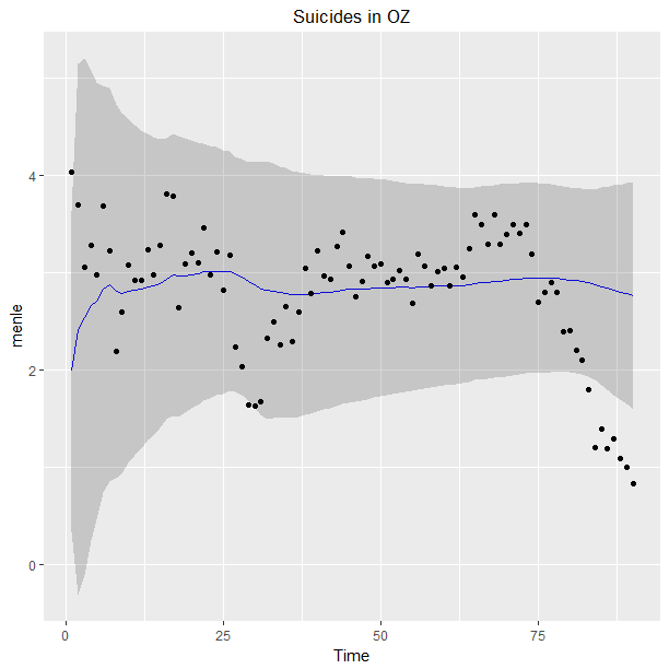
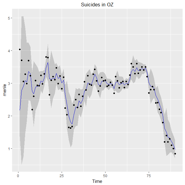
#Australian deaths
y=c(0.522, 0.425, 0.425, 0.477, 0.828, 0.616, 0.367, 0.431, 0.281,
0.465, 0.269, 0.578, 0.566, 0.508, 0.751, 0.681, 0.766, 0.456,
0.498, 0.419, 0.61, 0.457, 0.571, 0.348, 0.387, 0.582, 0.239,
0.237, 0.263, 0.424, 0.365, 0.375, 0.409, 0.389, 0.24, 0.159,
0.439, 0.509, 0.374, 0.434, 0.413, 0.329, 0.519, 0.549, 0.547,
0.496, 0.531, 0.596, 0.557, 0.573, 0.501, 0.543, 0.559, 0.691,
0.44, 0.568, 0.597, 0.474, 0.592, 0.598, 0.633, 0.606, 0.705,
0.481, 0.703, 0.701, 0.603, 0.698, 0.598, 0.802, 0.602, 0.599,
0.603, 0.702, 0.5, 0.498, 0.498, 0.6, 0.334, 0.274, 0.321, 0.541,
0.405, 0.289, 0.328, 0.313, 0.258, 0.214, 0.186, 0.159

Sequential Updates data and code

omega=.5  #The forgetting parameter.
i=0;m=1;n=1;a=2;b=1;
mn=rep(0,length(y)); uq=rep(0,length(y));lq=rep(0,length(y))
while (i<length(y))
{
  i=i+1
  a0=omega*a
  b0=omega*b
  m=m0+(1/(1+n0))*(y[i]-m0)
  n=n0+1
  a=omega*a0+.5
  b=omega*b0+(.5*n0)/(n0+1) *(y[i]-m0)^2

  mn[i]=qnorm(.5,m0,sqrt(b0/a0))
  uq[i]=qnorm(.95,m0,sqrt(b0/a0))
  lq[i]=qnorm(.05,m0,sqrt(b0/a0))

  m=m1;n=n1; a=a1; b=b1
}

Predicting ahead without forgetting

Figure 4.4: Link, Caption: Note without forgetting the precision of the predictions just increase

Predicting ahead with forgetting

Figure 4.5: Link, Caption: Here we allow forgetting so that posterior to prior precision is lost. This means that more weight is given to the current observation and less to the information stored in the prior.

4.2 The Normal distribution

The Normal distribution

The Normal distribution

The two parameter exponential family

4.2.1 The normal distribution with improper priors

The normal distribution with improper priors

The normal distribution with improper priors

The marginal posterior of μ

The marginal posterior of μ

The distribution of a future observation (The predictive)

The distribution of a future observation (The predictive)

4.2.2 The fully conjugate Normal-gamma prior

Using the fully conjugate, four parameter Normal-gamma prior

The fully conjugate, four parameter Normal-gamma prior

The fully conjugate, four parameter Normal-gamma prior

The fully conjugate, four parameter Normal-gamma prior

The fully conjugate, four parameter Normal-gamma prior

The predictive

Derivation of four parameter updates

Derivation of four parameter updates

Updates of the sufficient statistics for the fully conjugate model

Updates of the sufficient statistics for the fully conjugate model

Sequential updates to the sufficient statistics

Sequential Updates data and code

Sequential Updates data and code

Predicting ahead without forgetting

Predicting ahead with forgetting

The marginal posterior of $\mu$

The marginal posterior of $\mu$