4.1 The Multinomial dirichlet family

atgagcgccgttcccgatatccccggcggccccgcgcagcggctggc
ccaggcctgcgatgcgctgcgattgccggccgacgccggccagcagc
agaagctgctgcgctatatcgagcaaatgcagcgctggaaccgcacg
tacaacctgactgccatccgggatccggggcagatgctcgtgcagca
cctgttcgacagtctgtcggtcgtggcgccgctggagcgtggcctgc
ccggcgtggtgctggccatcatgcgcgcccattgggacgtcacatgc
gtggacgcagtcgagaagaaaaccgcattcgtgcgacagatggccgg
cgcgctcggactgcccaatctgcaggccgcgcatacccgtatcgaac
agctcgaaccggcgcaatgcgacgtggtgatatcgcgtgcgttcgct
tcgttacaggacttcgcgaagctggccggccgccacgtgcgcgaggg
tggtaccctcgtcgccatgaagggcaaggtgcccgatgacgaaatcc
aggcgttacagcaacacggccactggacggtcgaacggatcgaaccg
ttggtggtgccggcactcgacgcgcaacgctgcctgatatggatgcg
acgcagtcaaggaaacata

Suppose that $\text{𝐗}\sim \mathrm{Multinomial}(\mathrm{N},𝜽)$ is a $p$-dimensional sampling distribution then we can express the multinomial density as

$f(\text{𝐱}\mid 𝜽)=N!{\displaystyle \prod _{j=1}^p}{\displaystyle \frac{{\theta }_j^{x_j}}{x_j!}},$

where $N={\sum }_{j=1}^p{x}_j$ and ${\sum }_{j=1}^p{\theta }_j=1$. Note that this is from the multi-parameter exponential distribution shown by Equation (4.1) with $T(x)=\left[\begin{array}{c}\hfill x_1\hfill \\ \hfill x_2\hfill \\ \hfill \mathrm{⋮}\hfill \\ \hfill x_p\hfill \end{array}\right]$ and $\eta (\theta )=\left[\begin{array}{c}\hfill \log ({\theta }_1)\hfill \\ \hfill \log ({\theta }_2)\hfill \\ \hfill \mathrm{⋮}\hfill \\ \hfill \log ({\theta }_p)\hfill \end{array}\right]$

Suppose that $𝜽\sim \mathrm{Dirichlet}(𝜶)$ where $𝜽=\{{\theta }_1,{\theta }_2,\mathrm{\dots },{\theta }_p\}$ and ${\sum }_{j=1}^p{\theta }_j=1$ then we can express the Dirichlet distribution as

$\pi (𝜽)$

$={\displaystyle \frac{1}{\text{𝐁}(𝜶)}}{\displaystyle \prod _{j=1}^p}{\theta }_j^{{\alpha }_j-1}$

where ${\alpha }_j$ can be counts and $\text{𝐁}(𝜶)=\frac{{\prod }_{j=1}^p\mathrm{\Gamma }({\alpha }_j)}{\mathrm{\Gamma }({\sum }_{j=1}^p{\alpha }_j)}$ is the normalising constant.

It is easy to see that these two distributions are conjugate because

	$\pi (𝜽\mathbf{\mid }\text{𝐱})$	$\propto \pi (𝜽)f(\text{𝐱}\mid 𝜽)$
		$\propto {\displaystyle \prod _{j=1}^p}{\theta }_j^{{\alpha }_j-1}\times {\displaystyle \prod _{j=1}^p}{\theta }_j^{x_j}$
		$\propto {\displaystyle \prod _{j=1}^p}{\theta }_j^{{\alpha }_j+x_j-1}$
	$⟹𝜽\mathbf{\mid }\text{𝐱}$	$\sim \mathrm{Dirichlet}({\alpha }_1+x_1,{\alpha }_2+x_2,\mathrm{\dots },{\alpha }_p+x_p)$
		$\sim \mathrm{Dirichlet}(𝜶+\text{𝐱})$

The marginal parameters of the Dirichlet are marginally Beta as described below

	$({\theta }_1,{\theta }_2\mathrm{\dots },\mathrm{\dots },{\theta }_p)$	$\sim \mathrm{Dirichlet}({\alpha }_1,{\alpha }_2\mathrm{\dots },\mathrm{\dots },{\alpha }_p)$
	$⟹{\theta }_j$	$\sim \text{Beta }({\alpha }_j,{\sum }_{i\ne j}{\alpha }_i),j=1,2,\mathrm{\dots },p.$

The number of taxis that pass per minute over a 50 minute interval are recorded as:

If the events of taxis passing can be assume iid and from a Poisson distribution. Find the expected rate of a arrival and a 95% CI for that rate of arrival assuming anon-informative prior for $\lambda$.

1. 1.

   What is the posterior probability of the proportion of DNA bases shown below given a non-informative prior?

2. 2.

   What are the marginal distributions ie $\pi (a\mid x),\pi (c\mid x),\pi (g\mid x),\pi (t\mid x)$?

atgagcgccgttcccgatatccccggcggccccgcgcagcggctggcccaggcctgcgatgcgctgcgattgccggccgacgccggccagcagc
agaagctgctgcgctatatcgagcaaatgcagcgctggaaccgcacgtacaacctgactgccatccgggatccggggcagatgctcgtgcagca
cctgttcgacagtctgtcggtcgtggcgccgctggagcgtggcctgcccggcgtggtgctggccatcatgcgcgcccattgggacgtcacatgc
gtggacgcagtcgagaagaaaaccgcattcgtgcgacagatggccggcgcgctcggactgcccaatctgcaggccgcgcatacccgtatcgaac
agctcgaaccggcgcaatgcgacgtggtgatatcgcgtgcgttcgcttcgttacaggacttcgcgaagctggccggccgccacgtgcgcgaggg
tggtaccctcgtcgccatgaagggcaaggtgcccgatgacgaaatccaggcgttacagcaacacggccactggacggtcgaacggatcgaaccg
ttggtggtgccggcactcgacgcgcaacgctgcctgatatggatgcgacgcagtcaaggaaacata

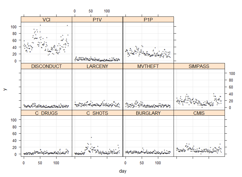
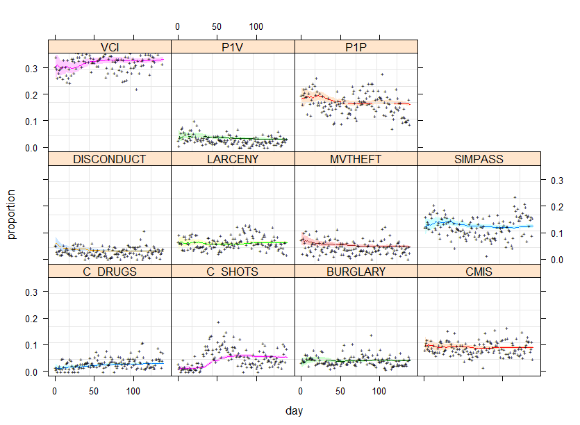
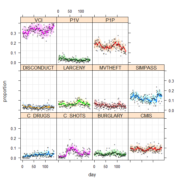
Instead of $𝜽$ and $N$ being fixed, we assume that both change over time:

${\text{𝐗}}_t\sim \mathrm{Multinomial}({\mathrm{N}}_{\mathrm{t}},{𝜽}_{\mathrm{t}})$. The sequential updates of the hyper-parameters of ${𝜽}_t$ are very straightforward. Let ${𝜶}_t$ be the sufficient statistics $𝜶=\{{\alpha }_1,{\alpha }_2,\mathrm{\dots },{\alpha }_p\}$ on day $t$ and ${\text{𝐱}}_t$ be the crime statistics on day $t$.

${𝜶}_t\leftarrow {𝜶}_{t-1}+{\text{𝐱}}_t$

where $t=1,2,\mathrm{\dots }N$

#R code for sequential updates of alpha.

alpha=rep(1,P); mn=matrix(0,N,P); uq=matrix(0,N,P)
lq=matrix(0,N,P);uq=matrix(0,N,P)
while (t<N)
{
  i=i+1
  alpha=alpha+as.numeric(y[i,])
  mn[t,]=qbeta(rep(.5,P),p1,sum(alpha)-alpha)
  uq[t,]=qbeta(rep(.995,P),p1,sum(alpha)-alpha)
  lq[t,]=qbeta(rep(.005,P),p1,sum(alpha)-alpha)
}