Chapter 3 Week 3: Bayesian statistics: Prediction

One of the primary purposes of statistics is to predict future values. The validity of a model can be assessed by seeing how accurately the model predicts. Bayesian statistics has a principled way of doing this.

The essential point is that there are two sources of uncertainty (dispersion) in predictions

• •

  Uncertainty in the parameter values; (Expressed by the posterior)

• •

  Uncertainty due to the fact that any future value is itself a random event (Sampling uncertainty expressed through the likelihood).

In classical statistics it is usual to fit a model to data, and then make predictions of future values on the assumption that this model estimate is known exactly, the so–called estimative approach. That is, only sample uncertainty is needed to explain the uncertainty of a a prediction. There is no completely satisfactory way around this problem in the classical framework since parameters are not thought of as being random.

Ted is the football team’s new goalkeeper. He predicts that he can save any number of goal attempts. To test him out on his claim some of the team ($n=5$ players) test his ability at a staged penalty shoot out. Ted saves 5 goals in a row.

Let $\pi$ be the probability of Ted making a save. The statistical question is the testing of Ted’s assertion that he has a 100% chance of making a save or $p(\pi )=1.$

The classical estimate of $\pi$ is $\widehat{\pi }=\frac{\sum x_i}{n}$ where $x_i=1$ denotes a save and $x_i=0$ a goal. The standard error of $\widehat{\pi }$ can be estimated by the expression $\sqrt{\frac{\widehat{\pi }(1-\widehat{\pi })}{n}}.$

1. (a)

   Why could the classical analysis could lead to a questionable prediction about Ted saving the next goal? [2]

2. (b)

   Calculate the posterior distribution using Bayes theorem, the likelihood and a flat prior $p(\pi )=1$. Sketch the posterior. [ Hint: make sure the posterior distribution integrates to 1]

3. (c)

   What is the predictive probability that Ted will save the next goal? Why is this more sensible than the result obtained in (a)?

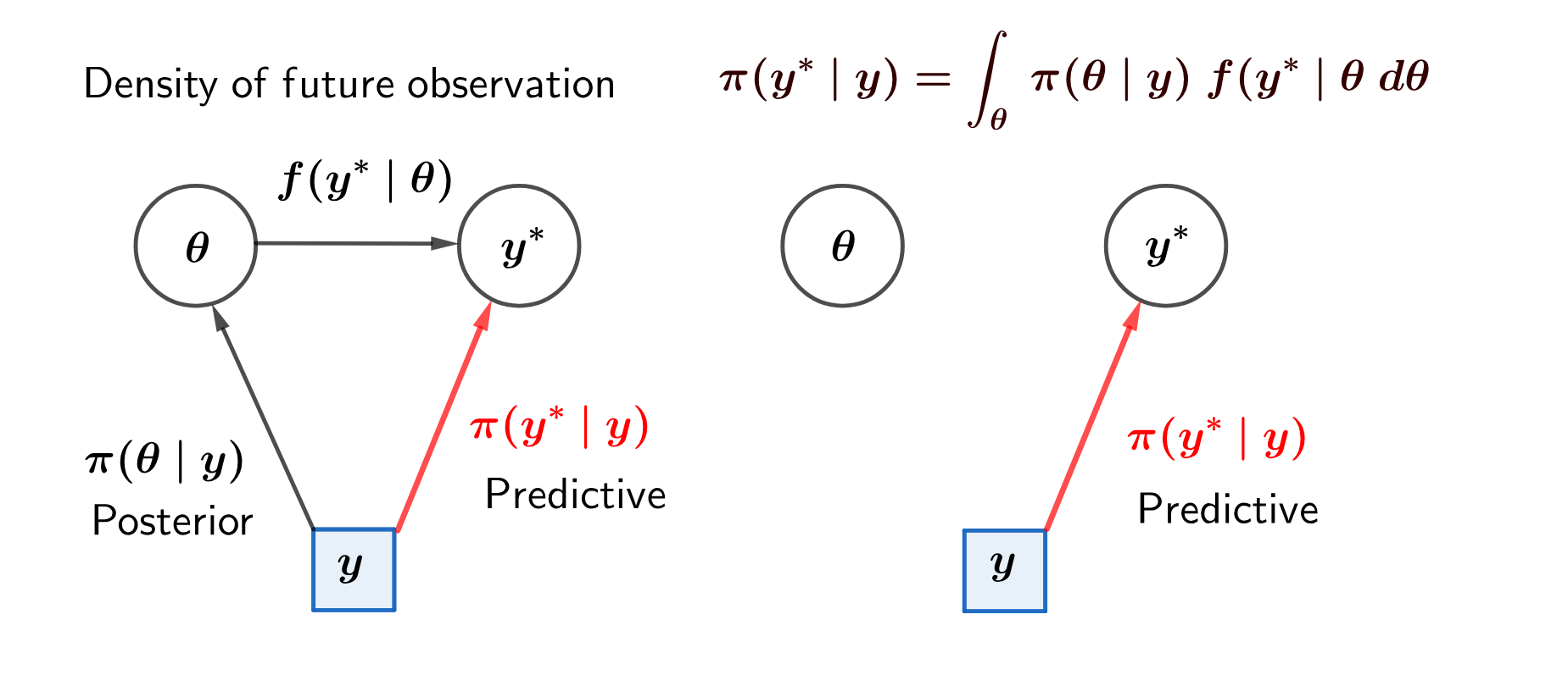
Within Bayesian inference it is straightforward to allow for both sources of uncertainty by simply averaging over the uncertainty in the parameter estimates, the information of which is completely contained in the posterior distribution.

So, suppose we have past observations $x=(y_1,\mathrm{\dots },y_n)$ of a variable with density function (or likelihood) $f(y|\theta )$ and we wish to make inferences about the distribution of a future value of a random variable $Y^{*}$ from this same model. With a prior distribution $\pi (\theta )$, Bayes’ theorem leads to a posterior distribution $\pi (\theta \mid y)$. Then the predictive density function of $y^{*}$ given $y$ is: