Home page for accesible maths 12 Introduction to Likelihood Inference 15.3 Summary 12.2 What is likelihood?

Style control - access keys in brackets

Font (2 3) - + Letter spacing (4 5) - + Word spacing (6 7) - + Line spacing (8 9) - +

12.1 Motivation

TheoremExample 12.1.1 London homicides

A starting point is typically a subject-matter question.

Four homicides were observed in London on 10 July 2008.

Is this figure a cause for concern? In other words, is it abnormally high, suggesting a particular problem on that day?

We next need data to answer our question. This may be existing data, or we may need to collect it ourselves.

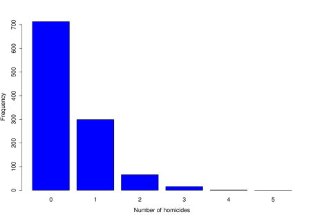
We look at the number of homicides occurring each day in London, from April 2004 to March 2007 (this just happens to be the range of data available, and makes for a sensible comparison). The data are given in the table below.

No. of homicides per day	0	1	2	3	4	$\geq 5$
Observed frequency	713	299	66	16	1	0

Table 12.1: Number of homicides per day over a 3 year period.

Before we go any further, the next stage is always to look at the data through exploratory analysis.

⬇

> obsdata<-c(713,299,66,16,1,0)

> barplot(obsdata,names.arg=0:5,xlab="Number of homicides", ylab="Frequency",

col="blue")

Next, we propose a model for the data to begin addressing the question.

It is proposed to model the data as iid (independent and identically distributed) draws from a Poisson distribution.

Why is this a suitable model?

What assumptions are being made?

Are these assumptions reasonable?

The probability mass function (pmf) for the poisson distribution is given by

{\color[rgb]{1,1,1}\Pr[X=x]=\frac{\lambda^{x}\exp(-\lambda)}{x!},}

for $x=0,1,2,\dots$ , so it still remains to make a sensible choice for the parameter $\lambda$ . As before, we will make an estimate of $\lambda$ based on our data; the equation we use to produce the estimate will be a different estimator than in Part 1.

12.2 What is likelihood?

In the last example we discussed that a model for observed data typically has unknown parameters that we need to estimate. We proposed to model the London homicide data by a Poisson distribution. How do we estimate the parameter? In Math104 you met the method of moments estimator (MOME); whilst it is often easy to compute, the estimators it yields can often be improved upon; for this reason it has mostly been superceded by the method of maximum likelihood.

Definition.

Suppose we have data $x_{1},\ldots,x_{n}$ , that arise from a population with pmf (or pdf) $f(\cdot)$ , with at least one unknown parameter $\theta$ . Then the likelihood function of the parameter $\theta$ is the probability (or density) of the observed data for given values of $\theta$ .

If the data are iid, the likelihood function is defined as

L(\theta|x_{1},\ldots,x_{n})=\prod_{i=1}^{n}f(x_{i}|\theta).

The product arises because we assume independence, and joint probabilities (or densities) obey a product law under independence (Math230).

TheoremExample 12.2.1 London homicides continued

For the Poisson example, recall that the probability mass function (pmf) for the Poisson distribution is given by

\Pr[X=x]=\frac{\lambda^{x}\exp(-\lambda)}{x!}.

We will always keep things general to begin by talking in terms of data $x_{1},\ldots,x_{n}$ , rather than the actual data from the table. From the above definition, the likelihood function of the unknown parameter $\lambda$ is

{\color[rgb]{1,1,1}L(\lambda|x_{1},\ldots,x_{n})=\prod_{i=1}^{n}\frac{\lambda^% {x_{i}}\exp(-\lambda)}{x_{i}!}.}

Let’s have a look at how the likelihood function behaves for different values of $\lambda$ . To keep things simple, let’s take just a random sample of 20 days.

⬇

set.seed(1)

#read in the data

x<-c(rep(0,713),rep(1,299),rep(2,66),rep(3,16),4)

%\end{lstlisting}

\begin{lstlisting}

#take a sample: 20 observations

xs<-sample(x,20)

⬇

#likelihood function

L<-function(lam){

m<-length(lam)

sapply(1:m, function(i) prod(dpois(xs,lam[i])))

}

⬇

#values of lambda to plot (trial and error..)

lam<-seq(from=0.3,to=1.1,length=100)

plot(lam,L(lam),type="l")

What does the likelihood plot tell us?

Definition.

Maximum likelihood estimator/estimate. For given data $x_{1},\ldots,x_{n}$ , the maximum likelihood estimate (MLE) of $\theta$ is the value of $\theta$ that maximises $L(\theta|x_{1},\ldots,x_{n})$ , and is denoted $\hat{\theta}$ . The maximum likelihood estimator of $\theta$ based on random variables $X_{1},\ldots,X_{n}$ will be denoted $\hat{\theta}(\bf{X})$ .

So the MLE, $\hat{\theta}$ , is the value of $\theta$ where the likelihood is the largest. This is intuitively sensible.

It is often computationally more convenient to take logs of the likelihood function.

Definition.

The log-likelihood function is the natural logarithm of the likelihood function and, for iid data $x_{1},\ldots,x_{n}$ is denoted thus:

	$\displaystyle l(\theta\|x_{1},\ldots,x_{n})=\log\{L(\theta\|x_{1},\ldots,x_{n})\}$	$\displaystyle=\log\left\{\prod_{i=1}^{n}f(x_{i}\|\theta)\right\}$
		$\displaystyle=\sum_{i=1}^{n}\log\left\{f(x_{i}\|\theta)\right\}.$

One reason that this is a good thing to do is it means we can switch the product to a sum, which is easier to deal with algebraically.

IMPORTANT FACT: Since ‘log’ is a monotone increasing function, $\hat{\theta}$ maximises the log-likelihood if and only if it maximises the likelihood; if we want to find an MLE we can choose which of these functions to try and maximise.

Let us return to the Poisson model. The log-likelihood function for the Poisson data is

	$\displaystyle l(\lambda\|\bf{x})$	$\displaystyle=\sum_{i=1}^{n}\log\left\{\frac{\lambda^{x_{i}}\exp(-\lambda)}{x_% {i}!}\right\}$
		$\displaystyle=\sum_{i=1}^{n}\left\{\log(\lambda^{x_{i}})+\log(\exp(-\lambda))-% \log(x_{i}!)\right\}$
		$\displaystyle=\sum_{i=1}^{n}\left\{x_{i}\log(\lambda)-\lambda-\log(x_{i}!)\right\}$
		$\displaystyle=\log(\lambda)\sum_{i=1}^{n}x_{i}-n\lambda-\sum_{i=1}^{n}\log(x_{% i}!).$

We can now use the maximisation procedure of our choice to find the MLE. A sensible approach in this case is differentiation.

{\color[rgb]{1,1,1}\frac{\partial}{\partial\lambda}l(\lambda|{\bf x})=\frac{1}% {\lambda}\sum_{i=1}^{n}x_{i}-n.}

Now if we solve $\frac{\partial}{\partial\lambda}l(\lambda|{\bf x})=0$ , this gives us potential candidate(s) for the MLE. For the above, there is only one solution:

\displaystyle{\color[rgb]{1,1,1}\hat{\lambda}^{-1}\sum_{i=1}^{n}x_{i}-n=0}

i.e.

\displaystyle{\color[rgb]{1,1,1}\hat{\lambda}=\frac{\sum_{i=1}^{n}x_{i}}{n}=% \bar{x}.}

To confirm that this really is the MLE, we need to verify it is a maximum:

\frac{\partial^{2}}{\partial\lambda^{2}}l(\lambda|{\bf x})=-\lambda^{-2}\sum_{% i=1}^{n}x_{i}<0.

It is clear intuitively that this is a sensible estimator; let’s formalise that into two desirable features we may look for in a ‘good’ estimator. We recall these properties (which you have met before):

Now plugging in the value of $\bar{x}$ we find that

\hat{\lambda}=\frac{(0\times 713)+(1\times 299)+(2\times 66)+(3\times 16)+(4% \times 1)}{713+299+66+16+1}=\frac{483}{1095}.

Plugging in the actual numerical values of the data at the last minute is good practice, as it means we have solved a more general problem, and helps us to remember about sampling variation.

The next step is to check that the Poisson model gives a reasonable fit to the data.

Plotting the observed data against the expected data under the assumed model is a useful technique here.

⬇

> #value of lambda from mom

> momlam<-483/1095

> #expected data counts

> expdata<-1095*dpois(0:5,momlam)

> #make plot

> barplot(rbind(obsdata,expdata),names.arg=0:5,xlab=

"Number of homicides",ylab="Frequency"

col=c("blue","green"),beside=T)

> #add legend

> legend("topright",c("observed","expected"),

col=c("blue","green"),lty=1)

The fit looks very good!

Let us now compare this to another estimator you already know: the method of moments estimator from Math104.

Definition.

Let $X_{1},\ldots,X_{n}$ be an iid sample from pmf or pdf $f(\cdot|\theta)$ , where $\theta$ is one-dimensional. Then the method of moments estimator (MOME) $\hat{\theta}$ solves

\mathbb{E}_{\hat{\theta}}[X]=\frac{1}{n}\sum_{i=1}^{n}X_{i}.

The left hand side is the theoretical moment and the right hand side is the sample moment. What this means is that we should choose the value of $\hat{\theta}$ such that the sample mean is equal to the theoretical mean.

In our example, recall that for a Poisson distributed random variable, $\mathbb{E}[X]=\lambda$ . Therefore the MOME for $\lambda$ is

\hat{\lambda}=\frac{1}{n}\sum_{i=1}^{n}X_{i}.

Notice that the MLE coincides with the MOME. We should be glad it does in this case, because the estimator is clearly sensible!

Whenever the MOME and MLE disagree, the MLE is to be preferred. Much of the rest of this part of the course sets out why that is the case.

Finally, we need to provide an answer to the original question.

Four homicides were observed in London on 10 July 2008. Is this figure a cause for concern?

The probability, on a given day, of seeing four or more homicides under the assumed model, where $X\sim\operatorname{Poisson}(\hat{\lambda}=\frac{483}{1095})$ , is given by

\displaystyle{\color[rgb]{1,1,1}\Pr[X\geq 4]=1-\Pr[X<4]=0.0011}

by Math230 or R.

But what must be borne in mind is that we can say this about any day of the year.

Assuming days are independent (which we did anyway when fitting the Poisson distribution earlier), if $Y$ is the number of times we see 4 or more homicides in a year, then $Y\sim\operatorname{Binomial}(365,0.0011)$ , and

\displaystyle{\color[rgb]{1,1,1}\Pr[Y\geq 1]=1-\Pr[Y=0]=0.33.}

So there is a chance of approximately $1/3$ that we see 4 or more homicides on at least one day in a given year.

Some R code for the above:

⬇

> #P[X>=4]:

> ans1<-1-ppois(3,momlam)

> #P[Y>=1]:

> ans2<-1-dbinom(0,365,ans1)