This blog will give you a simple and general insight into one of the dimensionality reduction technique – Principle component analysis (PCA). We assume our reader has basic knowledge of PCA and want to understand its principle visually.
Nowadays, millions of data generated every second. There is a common phenomenon in data structure: High dimension. Under such a scenario, explore, visualize and analyse data is hard and time-consuming. Thus, our objective is to find a low-dimensional representation of data that captures as much relevant/interesting information, which is dimensionality reduction (i.e, reduce 3 dimensions to 2 dimensions as the figure below).

What is Principle Component Analysis?
PCA is one of most widely used tools in dimensionality reduction. It could reduce \( m \) variables into \( k \) principle components ( \( m>>k \)), and each component is a linear combination of original variables. That’s why PCA belongs to linear dimensionality reduction. In mathematics, denote \(X_1,X_2,…,X_d \) as \(d\) dimensional variables in dataset, our aim is to find \(j\) components that satisfied: \(Z_j = \phi_{j,1}X_1+\phi_{j,2}X_2+…+\phi_{j,d}X_d\).
\(\phi_{j,1}\) describe the weights assigned to original variable \(X_1\) for principle \(Z_j\). That is how much information of \(X_1\) is assigned to the \(j\) principle. This could be used to explain the meaning of each principle.
How to understand visually?

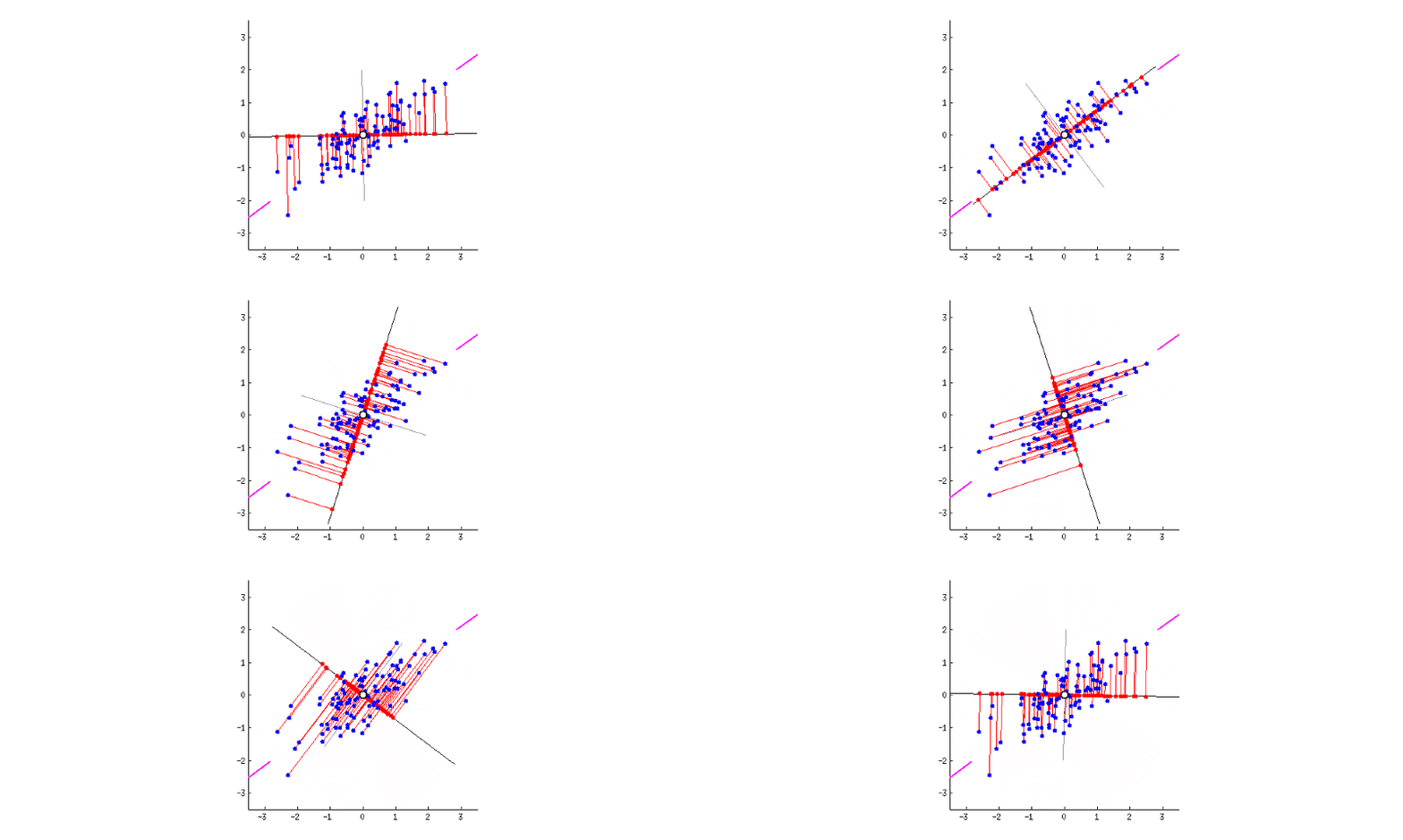
GIF above shows reducing two dimensions to 1 dimension. We could see that the shape of data is an ellipse.
Currently, we have two dimensions: x-axis and y-axis. Now we are trying to reduce them to 1-dimension which has as much information. This means, instead of the two axises, we will express our data in one new axis.
- Firstly we have to standardise the data, so the new origin of axes is located in the centre of the ellipse.
- Next, we have to rotate the new axis to find the new dimension as we could see the new axis is rotated 360 degrees. How to decide where should the new axis locate? Recall that, we want the new reduced dimension to capture as much relevant/interesting information. So, the new axis should locate in the direction which has as much information as possible – largest variance! That is to say, the larger the variance, the more important the data of this dimension is the principal component. The smaller the variance, the less important this dimension (corresponding to the shorter the ellipse axis), then this dimension can be discarded. We could see in the GIF when the coordinate axis turns to coincide with the pink colour, the projection points of each point on the first coordinate axis are the most dispersed.
- That’s all done! In this 2-d example, we have reduced 2 dimensions to 1 dimension. It could be easily extended to high dimensions.
Extra information
PCA is easier to use, it has lots of advantages:
- Only measure the information through the variance, and do not affect by other factors.
- The orthogonality between the principal components can eliminate the mutual influence factors between the original data components.
- It is efficient and effective in implementation.
However, it still has some disadvantages:
- It may be hard to explain the meaning of the new principle. If the model is used to explain, the choice and explanation of principles should be careful.
- Non-principal components with small variance may also contain important information about sample differences, and discarding may be unwise due to dimensionality reduction.
- It is based on the Euclidean distance, which is suitable for numerical data. However, if there are categorical data or ordinal/nominal information behind the data, PCA based on Euclidean distance may not be suitable.
Other supplement:
How to implement the PCA in R could read:
https://rpubs.com/jormerod/594859
The specific mathematical process could be found with example:
https://towardsdatascience.com/the-mathematics-behind-principal-component-analysis-fff2d7f4b643
Feel free to leave me message below: