
Learning is an essential part of life, which we do both consciously and subconsciously. From an early age we humans are usually expected to attend school and study. This social custom was introduced hoping that we can start learning about a wide range of topics as early as possible. This form of learning where we intentionally try to change our competences, attitudes and/or knowledge fits into the category of conscious learning (Simons 2012). However, there exists another form of learning. One which we are not fully aware of and ‘naturally’ happens through the interactions we experience with our environment
It is only natural that the ideas behind reinforcement learning are relevant when looking at states that evolve through time. For example, looking at the evolution of rubber tree plants within the Amazon rainforest. In the 1950s Richard Bellman found a way to break these down as to obtain a single value representing the payoff from making a specific decision in terms of both the immediate reward and future discounted reward. These equations are know as the Bellman equations and rely on a so called action-value function. This represents a value of taking a certain action in a specific state. When the number of action and state pairs is very large we can not record each value and instead use a formula to approximate them when needed. This is called functional approximation.
The algorithm used to make the ‘best’ decision using reinforcement learning tries to minimise a loss function using gradient descent. In essence, by minimising we improve our machine’s ability to make good decisions. This is difficult to do directly, so we will use stochastic gradient descent. Fundamentally, this method approximates our problem and makes it easier to solve, however, when using this method we must compute something called a gradient and these gradients depend on other gradients. This nested structure makes it difficult to estimate. We use a process called backpropagation to solve this problem.
An example of backpropagation
Below is a short example from Domke (2011) illustrating why backpropagation works. This example is simple enough so that we
can clearly show each step of how backpropagation works.
Given a function f = exp(exp (x) + exp (x)^2 )+sin (exp (x) + exp (x)^2 ), we obtain the following expression for its derivative with respect to x:
\frac{df}{dx}=\exp{(\exp{(x)}+\exp{(x)}^2)}(\exp{(x)}+2\exp{(x)}^2)+ \cos{(\exp{(x)+\exp{(x)}^2})(\exp{(x)}+2\exp{(x)}^2)}.
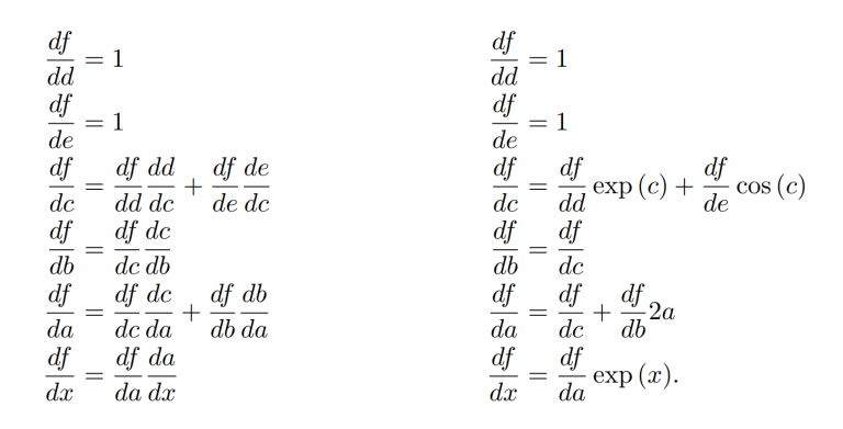
However, when the function f is a lot more difficult to differentiate we can use a different approach. By creating intermediate variables, we can differentiate them step by step and obtain the derivative of the function f. This is called backpropagation and works as follows. Let:
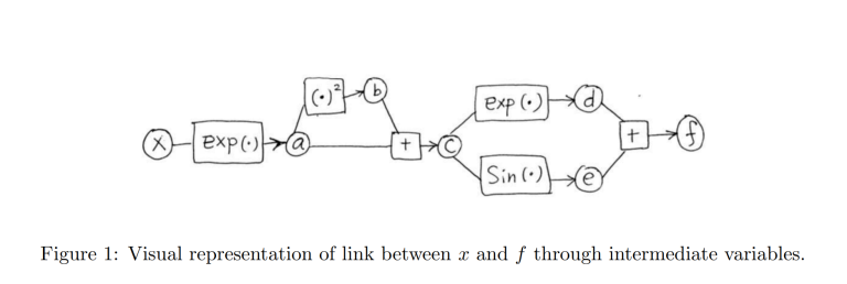
a = \exp{(x)} \\ b = a^2 \\ c = a+b \\ d = \exp{(c)} \\ e = \sin{(c)} \\ f = d+e.
Figure 1 gives a visual representation of the relationship between x and f linked by the intermediate variables created in equation above.
Finally, we can simply write the derivative of the intermediate terms using the chain rule work backwards until we obtain the derivative of f with respect to x.