
1. Introduction
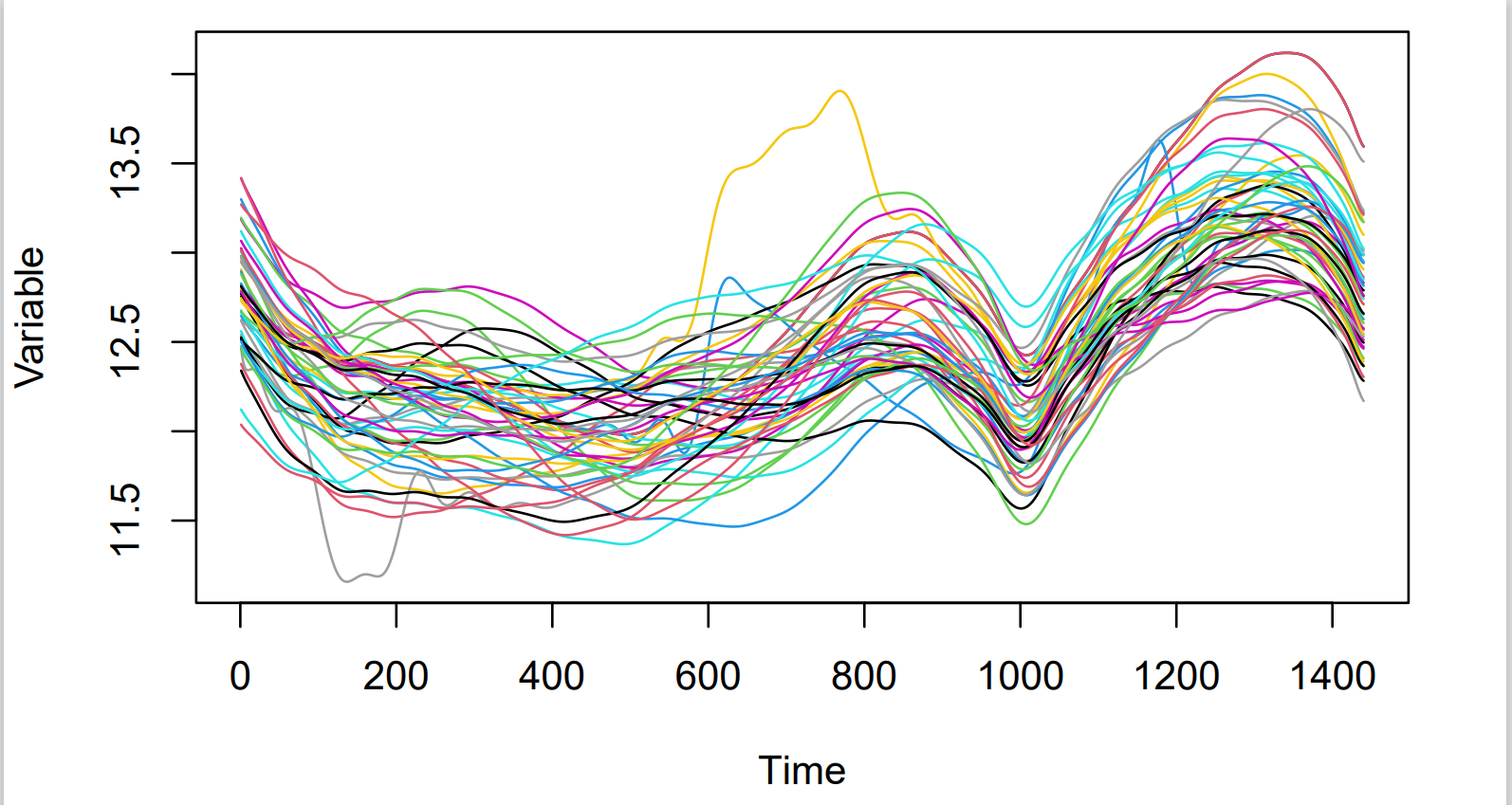
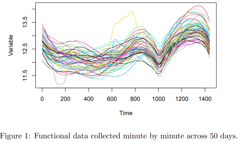
We call an anomaly, an observation that differs significantly from the rest of the data. These are important to detect as they can indicate the existence of a problem. Early identification could even prevent the problem recurring and avoid subsequently worse issues. There exist different types of anomalies; it may be a single observation that deviates from the rest, which is called a point anomaly or a group of points called a collective anomaly. In this blog however, we will be looking at anomalies in functional data. Figure 1 shows the data used, it consists of measurements made minute by minute across 50 days but we do not know what it measures. Hence, the two main types of anomaly will be, shape anomalies, which are curves that display a different behaviour than the other curves and magnitude anomalies, curves that at some point have a significant spike away from the rest of the curves. To detect these anomalies, we will look at two different methods. The total variation depth and modified shape similarity index (TVDMSS) and the functional outlyingness map using directional outlyingness (FOM(DO)), which methodology is discussed in Section 2. Then, Section 3 contains the results obtained from applying these methods to the data described and compares them. Finally, Section 4 contains the limitations of both methods and a general conclusion. Throughout this blog, the terms anomaly and outliers will be used interchangeably.
2. Methods
2.1 Total variation depth and modified shape similarity index
Since we are working with functional data, standard outliers detection techniques (for a single time series) will not be applicable. Here, outliers will have to be detected with respect to each curve. The following TVDMSS method is based on the work of Huang & Sun (2019). For each curves in our functional, data both the total variation depth (TVD) and modified shape similarity (MSS) are computed. The TVD can be interpreted as the total variability in the depth (along an interval of interest) of a curve compared to all other curves. At any given point in time, the deepest curve would be the one closest to the median of all curves at that point in time. The MSS is simply a measure of how similar the shape of a curve is compared to the shape of the all other curves. The lower the similarity the more likely it is to be considered an outlier.
Using these measures we can then start detecting anomalies. First, a classical boxplot is constructed using the MSS of each curve. An outlier corresponds to a curve for which the MSS is less than the P × 50% central region. Were the 50% central region corresponds to the 50% deepest curves. Outliers detected using this approach are considered shape outliers. Next, shape outliers are removed and a functional boxplot is constructed using the TVD. This functional boxplot is based on all the original curves prior to removing the shape outliers. Once again, the outlier detection region is Q × 50% central region. The RStudio function (tvdmss from the package fdaoutlier) used for this project allowed to independently modify the values of P, Q and the size of the corresponding central regions. Therefore, allowing the sensitivity detection level to be tuned. Outliers detected using the functional boxplot are considered magnitude outliers. In addition, for this blog, anomalies that characterise as both shape and magnitude outliers will also be highlighted, which the standard TVDMSS does not include. This was done by detecting magnitude anomalies while not removing shape anomalies.
2.2 Functional outlyingness map using directional outlyingness
A large number of outlier detection methods rely on using functional depths; as we just saw, this is true for TVDMSS. Dai & Genton (2019) argue that these might fall short of properly describing the centrality of functions and not detect anomalies characterised by their directional outlyingness. Therefore, using the work of Rousseeuw et al. (2018), Dai & Genton (2019) came up with the functional directional outlyingness which accounts for both the pointwise depth and the directional anomalies.
Outliers are detected using a functional outlier map (FOM). This is visually represented by a scatterplot displaying points and a cut-off line. If the points are out of the cut-off region they are considered outliers. The points are plotted using a functional directional outlyingness value on the x-axis; this reflects the total outlyingness of a given curve and the variation of the directional outlyingness on the y-axis; which represents the shape outlyingness of that curve. To fit this method, we used the function fOult from the R package mrfDepth. This function does not allow to change the level of anomaly detection, therefore, no tuning is possible for how strict we want to be with our anomalies.
3. Results
This section presents the results from applying the TVDMSS and FOM(DO) to the data presented in Figure 1.
3.1 Detecting anomalies using Total variation depth and modified shape similarity index
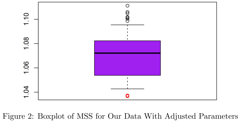
After manually tuning the TVDMSS algorithm to a level of detection which empirically seemed reasonable (P = 0.5 and Q = 1.1) we obtain the following results. As shown in Figure 2, three shape anomalies were detected using the classical boxplot of MSS. These are represented by the red circle below the boxplot.
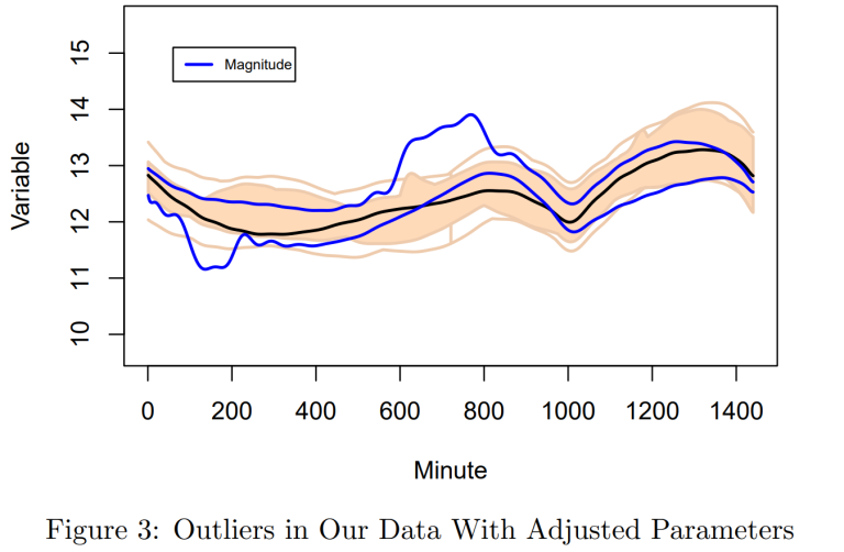
Next, the magnitude outliers were identified using the functional boxplot as seen in Figure 3. As we can see, two magnitude anomalies were detected, represented by the blue lines. The pale area corresponds to the 50% central region and the slightly darker lines are the anomaly thresholds.
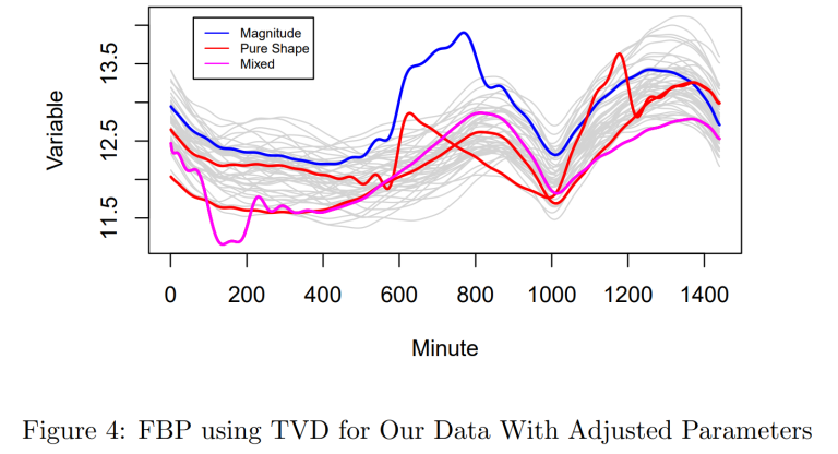
Finally, Figure 4 displays all the anomalies detected using the TVDMSS. We can see that one anomaly was classified as both a shape and magnitude anomaly. Furthermore, the shape anomaly detected by the boxplot of MSS corresponding to the lowest red line at t = 0 seems questionable. Empirically, it does not look very different from the other curves.
3.2 Detecting anomalies using functional outlyingness map using directional outlyingness
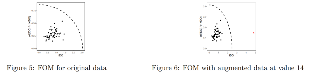
The FOM(DO) has not classified any of the curves as outliers. As shown in Figure 5, all the points lie within the cut-off line. As explained in Section 2.2, the function fOult used to create this cut-off line does not allow to modify the threshold level. Therefore, to test if the FOM(DO) would detect a more extreme outlier, a curve was added to the data with value 14 for all t. Figure 6 show that the FOM(DO) does detect this more severe outlier, which is represented by the red triangle. This was also tested with a curve at value 13, however, it was not detected as an outlier although it’s shape was very different from any other curve.
3.3 Comparing both anomaly detection methods
Comparing the results obtained by the two anomaly detection methods is limited by the R functions and packages that were used to produce them. Keeping that in mind, there are four major points on which these two can be compared. First, the TVDMSS algorithm was 10 times fast than running the FOM(DO), (0.05s vs 0.5). Secondly, the TVDMSS performances better when using the default values of the respective functions. Then, the FOM(DO) did not allow for any tuning, whereas this was easy for the TVDMSS. Therefore, once tuned the TVDMSS performed relatively well, by detecting all the true outliers.
4 Limitations and Conclusion
Both outlier detection methods have their respective limitations. Because of how the algorithm of the TVDMSS works, it favours shape over magnitude anomalies. Since shape anomalies are first detected then removed. This might be an issue for someone who is interested in anomalies that display both behaviours. This was therefore added as an extension to the TVDMSS, as discussed in Section 2.1. Another significant limitation of the TVDMSS is that it relies heavily on being tuned, the values of P, Q and the percentage size of the central region must be set using trial and error. Finally, the TVDMSS is based on both classical and functional boxplots, which themselves rely on sufficient sample size. For the FOM(DO), we have seen that it was not possible to tune the cut-off line to allow a less strict outlier detection threshold. However, there is also a theoretical limitation to its application in this project. The FOM(DO) performs well with multivariate functional data and although it does work in univariate cases, it does not have much power.
Therefore, we have seen that although both the TVDMSS and the FOM(DO) are two outlier detection methods which have strong theoretical founding, they both have the potential to detect shape and magnitude anomalies effectively. However, their performances is strongly affected by the context in which these are used and how they are implemented. For the data used in this project, the TVDMSS performed a lot better than the FOM(DO), almost perfectly detecting all three true outliers. Although, this is largely due to the inability to tune the FOM(DO). Therefore, it would be interesting to try and implement both these algorithms manually, enabling full control over the tuning of the parameters and thus re-evaluate their respective performances.