At STOR-i we are currently looking through our potential PhD projects. For each project we have been given a page summarizing the topic with some papers listed at the bottom. As I was looking through these papers I came across one which particularly interested me in an area I knew very little about. I decided a good way for me to form a deep understanding of this paper would be to write a blog post on it. This way you can learn something too.
The paper in question is called “A Tutorial on Bayesian Optimization”. So you may remember in a previous blog post I explored a Bayesian approach to a multi armed bandit problem and in another I looked at a heuristic approach to an optimization problem. Well today (or which ever day you decide to read this) we are looking at a Bayesian approach to an optimization problem.
So lets outline the situation. We have a function f(x). We would like to find the maximum of this function, however we do not know the structure of the function, and it is expensive to evaluate the function at certain points. Basically we have a black box which we give inputs (our x values) and receive an output (f(x) value). Since evaluating points of the function is expensive we can only look at a limited number of points in the function. So we have to decide which points to evaluate in order to find the maximum.
So how do we do this? Firstly we fit a Bayesian model to our function. We can then use this to formulate something called an acquisition function. The highest value of the acquisition function is the point we evaluate next.
Gaussian process regression is used to fit the Bayesian model. We suppose that f values of some x points are drawn at random from some prior probability distribution. This prior is taken by the Gaussian process regression as a multivariate normal with a particular mean and covariance matrix. A mean vector is constructed using a mean function at each x. The covariance is constructed using a kernel which is formulated so two x’s close together have a large positive correlation. This is due to the belief closer x’s will have similar function values. The posterior mean is then an average of the prior mean and an estimation made by the data with a weight dependent on the kernel. The posterior variance is just the prior covariance of that point minus a term that corresponds to the variance removed by observed values. The posterior distribution is a multivariate normal.

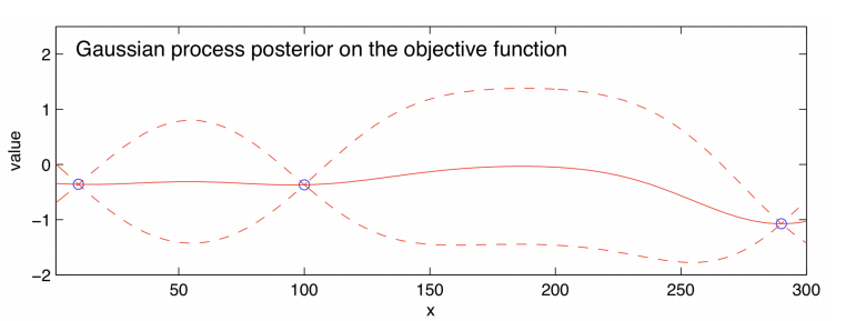
Illustrated above we have an estimate of the function f(x) (solid line) and the dashed lines show Bayesian credible intervals (these are similar to confidence intervals) with observed points in blue. Using this we can form an acquisition function such as:

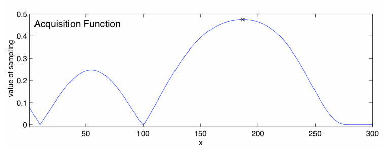
This function tells us which point of the equation to evaluate next. This is the maximum point of the function. There will be a balance between choosing points where we believe the global optimum and places with large amounts of variance.
There are many different types of acquisition functions. The most commonly used one is known as the expected improvement. In this case we assume we can only provide one solution as the maximum of f(x). So if we had no more evaluations left we would provide the largest point we have evaluated. However, if we did have just one more evaluation, our solution would remain the same if the new evaluation was no larger than the largest so far, but if the new evaluation is larger that would now be our solution. The improvement of the solution is the new evaluation minus the previous maximum. If this value is positive and zero otherwise. So when we choose our next evaluation we would like to choose one which maximizes improvement. It is not quite that simple as by the nature of the problem we do not know the value of an evaluation until we have chosen and evaluated that point. This is when we use a Bayesian model as we can use it to obtain the expected improvement of the points and then choose the point that has the largest expected improvement. This will choose points with high standard deviation and points with large means in the posterior distribution. This means there will be a balance between choosing points with high promise and points with large amounts of uncertainty.
This method can be applied to many problems including robotics, experimental particle physics and material design. This paper here explains the application of Bayesian optimization to the development of pharmaceutical products. To learn more I’d advice reading the paper I used for this blog as well as this paper which discusses constrained Bayesian optimization and its applications.
