This week it was time to choose which research topic, from the lectures that I mentioned last week, we would like to write our first report on. The topic I have decided on is: Network Modelling. While I was refreshing my memory on what was covered in the lecture, given by Chris Nemeth, I thought it would be a nice idea to give you some insight on the topic.
What is Network Modelling? It is statistical modelling using network data. But what is network data? I think the best way to explain it is with examples such as friends on Facebook or other social media, voting similarity of politicians, connections in the brain or even connections between people who have co-authored papers together.
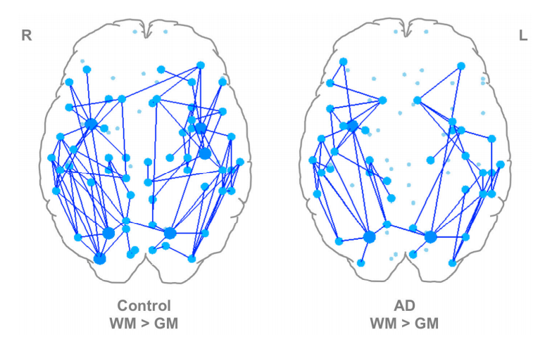
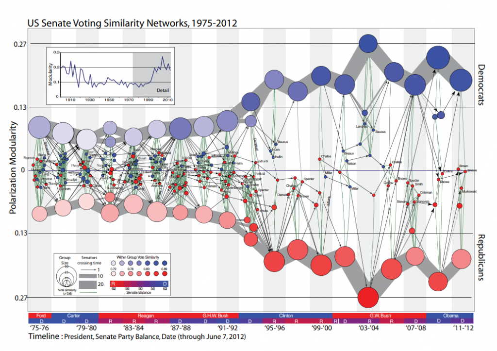
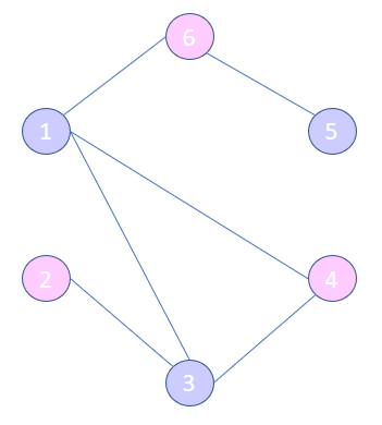
Before we go into the details let’s discuss the notation of a network. Here we have a basic network:
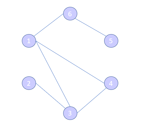
We can represent this network as a graph G=(V,E).
- V is a set of vertices in the network. So for this case we simply have V={1,2,3,4,5,6}. Depending on the network data vertices maybe named instead of just numbered.
- E is the set of edges. Each edge, e=(u,v) represents a connection between two vertices u and v. For this graph we have E={(1,3),(1,4),(1,6),(2,3),(3,4),(5,6)}.
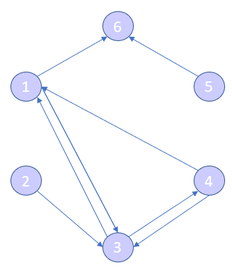
Different networks will require different information and so the graphs may look different:
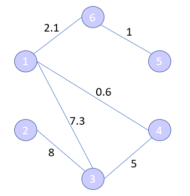
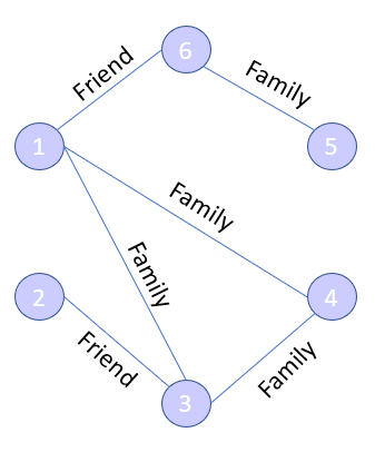
Graphs can also be represented as an adjacency matrices. The way I like to think of this matrix is that if there was a horizontal and vertical list of the vertices, then if there is an edge between the two vertices there will be a one in that slot of the matrix and a 0 if not. Here is what the adjacency matrix looks like for our example.
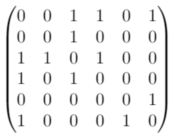
So, what can we do with this? Well by summing up the rows we can calculate the degree of each vertex. We can also calculate the edge density which is the number of edges (the sum of all the elements in the adjacency matrix over two) divided by all the possible edges. Also, we can calculate the average degree.
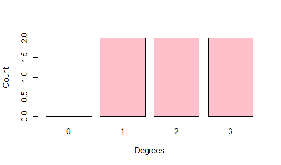
Using the adjacency matrix we can look at the degree distribution which gives us the proportion of nodes with a specific degree. This has a simple probability mass function such that the probability of a specific degree is the number of nodes with that degree divided by the total number of nodes. Degree distributions show us how many neighbours nodes have and how properties vary over a network.
So now we have explained the networks it is time to look at the modelling. The particular model we are going to look at today is Erdos-Renyi model. For a network, we have graph G(n,p) where n is the number of nodes and p is the probability of there being an edge between two nodes. This means we have a binomial probability mass function where each edge added is seen as a success. But how do we go about setting p? Real networks tend to be sparse. If you think about it the number of friends you have on Facebook is a very small proportion of the total number of people on Facebook. Not to say you don’t have many friends there is just a lot of people on Facebook. As the size of the network increases, p will decrease. So, if you think of Facebook only containing people you went to school with there would be a high probability of you being friends with any one person. But if you expand it to your town or your country or even the whole world it will decrease. So, one appropriate way to set p may be equal to a constant over the number of nodes. Like any model this model has criticisms. One main one being that each pair of nodes have the same probability of having an edge which clearly is unlikely in reality. You are more likely to be friends with someone if you are friends with all their friends. There are adaptations of this model that take that in to account which you can find in this book: A survey of statistical network models – Goldenberg, A., Zheng, A. X., Fienberg, S. E., & Airoldi, E. M. This book also details the Erdos-Renyi model.
