Currently as part of the MRes at STOR-i we are participating in lectures on research topics given by multiple lecturers. One I found particularly interesting was given by Adam M. Sykulski on work he is currently doing with a PhD student at STOR-i, Michael O’Malley, about most likely pathways in the ocean. So, lets dive right in. (I’m sorry, don’t worry there are no more puns.)
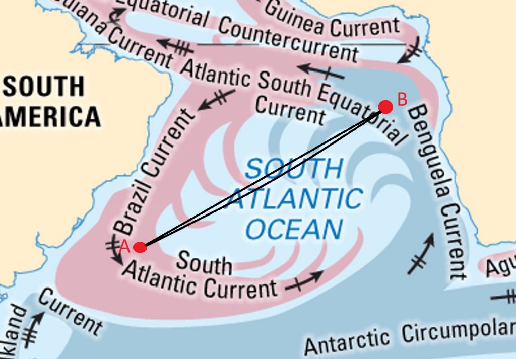
You may be confused by what is meant by this so I’m going to try and briefly explain it to you. Imagine you are a particle in the ocean at point A and you wish to end up at point B. This research finds the path you will most likely take.
So what path is this? Your first thoughts may be that you want the shortest path so a straight line. Then maybe you remember the world is spherical so that would a geodesic line. But also, you’re a particle in the ocean being pushed and pulled by the currents so maybe you follow them?

But why do we even want to know which path is most likely. The motivation behind this is biologic research conducted by Genoscope in France on genetic samples of zoo plankton at different points in the ocean and wanting to know how connected they are. It can also be used for studying the transport of things such as debris, plastic, or oil. So, we are trying to observe the connectivity between points in the ocean.
Before any statistical analysis can be done some data is needed. This data is gathered by the global drifter programme. Drifters (free-floating buoys) are released into the ocean and the path that they take is recorded and so we have data that can now be used.
But how do we use this data to find the most likely path between each point. It is very rare that a drifter will go through two particular points in the ocean. This means we can not just look at which paths the drifters take most frequently. Even if we try to connect paths of two drifters we can’t know that this is the most likely path.
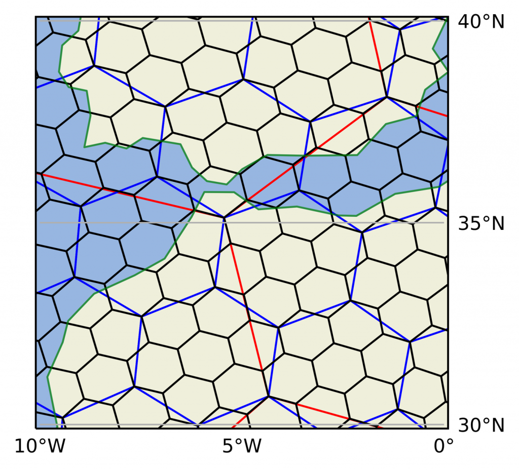
So, O’Malley and Sykulski have proposed a method to do this. To apply the method, they first decided on a method of splitting up the ocean into bins. This is used to define the probability of a particle going from one bin to another and determine the mostly likely path. Now an obvious choice would be to split it up into squares based on longitude and latitude. However, there are a few issues with this. Firstly, due to the earth being a sphere there are large variations of sizes in each square. As well, diagonal neighbours only share a vertex and no edges compared to other neighbours which share an edge and two vertices. So diagonal neighbours are disadvantaged. The method which has instead been used is a grid system named H3 by UBER. The advantages of this is that the bins the ocean is split into are fairly similar sizes and each neighbour shares an edge and two vertices.

Markov transition matrices are then formed using data from the drifters by looking at their location at each time step. For those that are not in the know, a Markov transition matrix is a matrix with elements pij which are the probability of transitioning from state i to j. In this instance each hexagon is a state. An important property for a Markov transition matrix is there is lack of memory between states. This means previous states don’t affect the probability of future states. The appropriate time step O’Malley and Sykulski have chosen is five days as this follows oceanographic literature. Dijkstra’s algorithm is then used to find the most likely path. I understand you may not be familiar with Dijkstra’s algorithm but all you need to know is that it is an algorithm to find the shortest path.

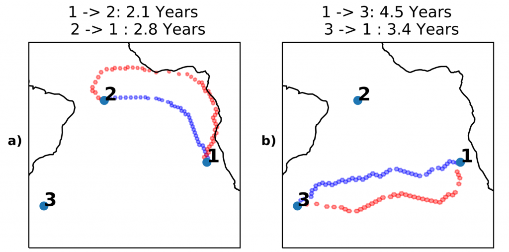
Now we have our most likely path what do we do with it? Well this research is trying to quantify the connectivity of two points in the ocean. To look at the full picture it is important to consider that currents at different points of the ocean are different speeds. So, to find this connectivity of points we look at the expected time taken to travel the most likely path.
It is hard to say what exactly about this lecture I found so interesting. I think its more than the fact I’ve always had a fondness for the ocean and is actually the elegance of the method which really grasped my focus. Which I would say is quite impressive for the third hour of an early morning three-hour lecture.
To learn more about this, definitely check out the paper which this blog is based upon: Estimating the travel time and the most likely path from Lagrangian drifters – Michael O’Malley, Adam M. Sykulski, Romuald Laso-Jadart and Mohammed-Amin Madoui
To learn more about Markov chains and transition matrices: Markov chains- James Robert Norris.
Or learn more about Dijkstra’s algorithm: “Chapter 10. Shortest Paths” Algorithms and Data Structures: The Basic Toolbox – Kurt Mehlhorn and Peter Sanders.
