Network Flow 🌊

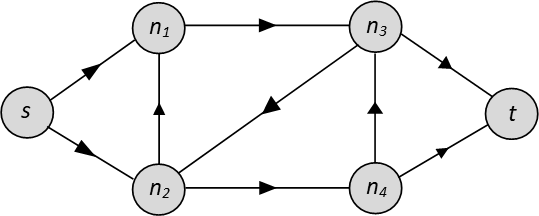
Everywhere we look, whether that’s in our social circles or at the electrical grid, we can see the existence of networks. In each network, we exchange or send some product from one point in the network to another point. This is what we define a flow network (or network flow) as, a collection of points on which we send a product (or flow) throughout this network. Formally, this can be represented by a graph like the one below.

Network with 6 nodes and 9 arcs (we call these arcs and not edges because they have a specific direction, e.g. water only travels one way down a pipe).

A good example of a flow network is a pipeline network. We have pipes going from pipeline junctions (things that connect pipes) to other pipeline junctions. These pipes and pipeline junctions form our network. The flow in our network would be water, flowing from one pipeline junction to the next through the pipes.

But we can imagine many things like networks. For example, the vehicle routing problem can be thought of as a network! Think of a company like Amazon, for which we’re all familiar with their next day delivery service. They’ll need to make hundreds of deliveries in a day to satisfy our privileged souls. The vehicle routing problem takes the Amazon delivery trucks (or any vehicle) and sets them the best routes to take in order to deliver all the parcels to our doorsteps in time whilst minimising delivery time and costs. Well take our houses as points on a graph for which the roads connect our houses together. This is a network! Then the flow we want to send from house to house are the parcels the trucks carry and want to deliver. So the vehicle routing problem, a common optimisation problem, can be thought of network flow problem!

Why do we want to think of problems as network flow problems? Because often they can get a lot easier to solve as flow networks! Let’s focus on a specific network flow problem…

The Maximum Flow Problem

Let two nodes (points) on the graph be special compared to the rest. Call one the source node and the other a sink node. The source node is the point at which all flow in the network starts from. The sink node is the point where all the flow ends up. The max-flow problem involves finding a flow through a network such that we get the maximum amount of flow going from the source node to the sink node.

Well this is an easy problem. The maximum amount of flow? The maximum is infinity so let’s just send an infinite amount of water through the pipes from the reservoir to our homes. Unfortunately for mathematicians, life is rarely so simple. Often, we aren’t able to send an infinite amount of flow through a network due to the capacities on the edges. For example, pipes can only hold finitely amount of water before they burst (and that’s when bad stuff happens).

Capacities aren’t the only thing we have to worry about. We impose this phenomenon known as flow conservation. This just means that, apart from the source and sink nodes, the total flow entering a node must equal the total flow leaving a node. Think of this like the law of conservation of energy, we can’t create or destroy flow throughout this network, we just transfer it.

The max-flow problem has been around for decades, dating back all the way to the 1950s when (some names) first introduced the problem to solve a Soviet transportation problem (cite some paper). As this has been around for years, there has been many approaches to solving the max-flow problem. These solutions generally come under two types; augmenting path algorithms and push-relabel algorithms. We’ll focus on augmenting path algorithms, specifically the original.

The Ford-Fulkerson Method

The Ford-Fulkerson method, published in 1956, was the first proposed method to solving the max-flow problem. The amazing thing about the Ford-Fulkerson method is that this method is guaranteed to give you the maximum flow of a network, if it stops.

So let’s learn how this method works! To do this, we need to learn about two things: residual networks and augmenting paths. To help us understand these concept, we’ll reference back to the flow network example in Figure 1 (copied below to avoid constant scrolling).

Residual networks

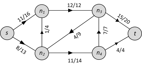
The word residual means remaining, or what’s leftover. What does this mean in terms of networks? Let’s take an arc from the network in Figure 1, say s → n₁. The current flow on this arc is 11, and the capacity (the maximum amount that can flow through this arc) is 16. Then we say the residual capacity on this arc is r_s,n₁ = 16 – 11 = 5, i.e. we can send an additional 5 units amount of flow through this arc. For another example, let’s look at the arc n₁ → n₃. The current flow in this arc is 12 and the capacity on this arc is also 12. This arc is currently working at maximum capacity, so we can’t send any more flow through this arc (because we don’t want any pipes to burst). Therefore the residual capacity on this arc is r_n₁,n₂ = 12 – 12 = 0.

Let’s look at arc n₁ → n₃ again. This arc is operating at maximum capacity, so we can’t send any more flow through this arc. But what if we’ve made a mistake and sent a bit too much flow through this arc and want to take it back? In real life, the the pipes only go in one direction. So if we send water down a pipe, we can’t send the water back through the same pipe. Luckily, as planners, we can cheat. Let’s create a ‘backwards pipe’, going from n₃ → n₁. This backwards pipe will represent the amount of flow we can subtract from the original pipe. So for arc n₁ → n₃, the flow on this arc is 12. Then for the backward arc n₃ → n₁, we say the residual capacity on this backward arc is 12, i.e. the amount of flow we can take back from the original arc. This little trick of creating ‘backward arcs’ is important and necessary because it allows us to ‘un-add’ flow and undo any work we do in case if make any mistakes, as well as to maintain flow conservation.

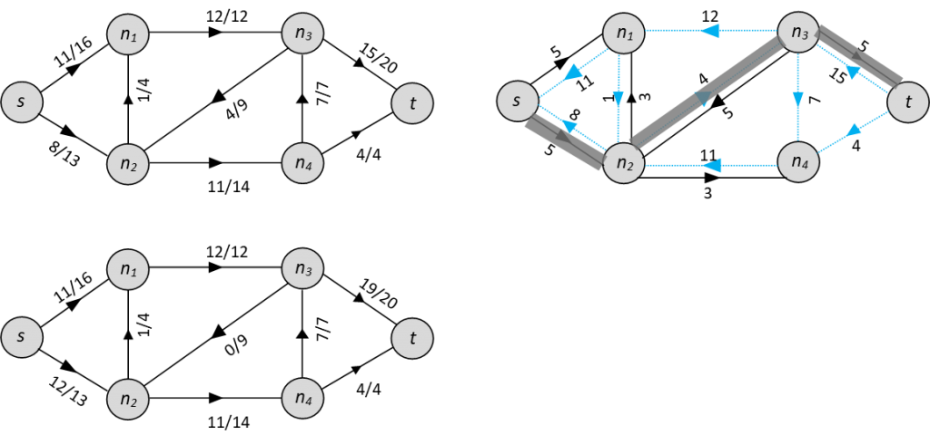
To conclude, the residual capacity for a forward (original) arc is the amount of additional flow we can send through the arc. The residual capacity for a backward arc is the amount of flow we can subtract from the forward arc. Then we define the residual network as the network with arcs with non-zero residual capacities. The residual network for the flow network in Figure 1 is shown below. The backward arcs are graphed as blue lines, just to emphasise that they aren’t real arcs in the original network.

Why do we even care about the residual network? Because the residual network shows us which arcs we can send more flow through. If we can’t send any more flow through an arc, then the residual capacity will be 0 and this arc just isn’t included in the residual network. Therefore, if we want to find the maximum flow to send through a network, we can use the residual network to see which arcs we can send more flow through. This nicely leads us onto augmenting paths.

Augmenting paths

The below picture depicts the process of selecting an augmenting path and augmenting the flow along this path. This process is described in more detail further on.

Figure 2. This picture shows the process of augmenting a flow. Start from the network in the top-left (this is the same network as Figure 1). The top-right shows the corresponding residual network with an augmenting path shaded. The bottom-left pic shows the network once we’ve augmented the flow along the selected augmenting path.

A path in a network is a sequence of arcs connecting two nodes together that doesn’t repeat any nodes (just so we don’t stuck in a never ending loop). For example, looking at Figure 1, a path from s to t could be s → n₁ → n₃ → t. Another path could be s → n₁ → n₃ → n₂ → n₄ → t.

Augmenting means to add. In terms of network flows, and particularly with the max-flow problem, we want to increase the flow in the network until we get the maximum flow possible. So an augmenting path in the network is a path where we can increase the flow along all arcs on this path. Well, if we’re looking for arcs where we can increase the flow through them, then let’s work with the residual network!

The residual network only includes arcs which we can send additional flow them, for which we can augment the flow along these arcs. The max-flow problem wants to send the maximum amount of flow from source node s to sink node t. So an augmenting path is a path from s to t in the residual network. For example, Figure 2 shows an augmenting path in the residual network (shaded).

So once we identify an augmenting path, how do we increase the flow? Look at the arcs on this path and their residual capacities. For the augmenting path in Figure 2, we have the augmenting path s → n₂ → n₃ → t. The residual capacities on these arcs tell us how much more flow we can add on these arcs before we reach maximum capacity. These residual capacities are 5, 4, and 5. We pick the smallest residual capacity, in this case 4. Then, in the original network, on the arcs of the augmenting path, increase the flow by 4. So, on the arc s → n₂, flow goes from 8 to 12. There is no arc n₂ → n₃ in the original network but remember, a backward arc represents a subtraction in the flow on the original arc. So to increase the flow on arc n₂ → n₃ means we decrease the flow on arc n₃ → n₂ from 4 to 0. Finally, on the arc n₃ → t, flow increases from 15 to 19. This process of increasing the flow is what we call augmenting flow.

The pseudocode (general steps) for the Ford-Fulkerson method is as follows:

1. Start with 0 flow in the network.

2. while there exists an augmenting path in the residual network from nodes s to t:

augment flow along the path in the original network

So the Ford-Fulkerson method will keeping running through the second step until there are no more augmenting paths. When there are no more augmenting paths, we can not increase the flow from nodes s to t anymore. Therefore, when this algorithm stops, we will have found the maximum flow of the network and have solved the max-flow problem for a given network.

Further Work

The Ford-Fulkerson method is one of the most commonly used methods to solving max-flow problems because of it’s simplicity to implement in real life and the guarantee that once the algorithm stops, you will have found the maximum flow of a network. However, this doesn’t mean it can’t be improved! The Ford-Fulkerson method is called a ‘method’ and not an ‘algorithm’ because it is very vague around how we find augmenting paths. Generally, augmenting paths are found randomly but if you have some specific method for finding these augmenting paths efficiently, then you can get to the solution a lot more efficiently and quickly. This is called improving on the computational complexity of an algorithm.

The Ford-Fulkerson method was published in 1956 (just a couple of years back) and so there have been MANY algorithms since then that have built upon and improved on this, such as the Edmonds-Karp algorithm. There are also a different class of algorithms, called the push-relabel algorithms, which tackles the max-flow problem in a different (more complicated but very interesting) way. And despite the max-flow problem being known since 1954 and many algorithms being published to solve this specific problem, there is still a lot of work being done in this area! Check out the links below for more details. Thanks for reading!