Heuristic search
A heuristic in the most common sense is a method involving adapting the approach to a problem based on previous solutions to similar problems. These approaches aim to be easily and quickly applicable to a range of problems, so as to find approximate solutions quickly without using the time and resources to develop and execute a precise approach. The principle of a heuristic can be applied to various problems in mathematics, science and optimsation by applying heuristics computationally.
Heuristic search is class of method which is used in order to search a solution space for an optimal solution for a problem. The heuristic here uses some method to search the solution space while assessing where in the space the solution is most likely to be and focusing the search on that area. It is often possible to model the process of solving a problem as a search through a solution space starting from an initial possible solution, with a method or set of rules dictating how to move from one possible solution to another. This method or rule set must be applied repeatedly in order to eventually satisfy some goal condition which indicates that a solution has been found. Often, this means assessing which path through the solution space improves the solution the most at each iteration of the applied method and choosing this. For more information, see here.
Searching solution spaces has been integral for the development of artificial intelligence for problem solving. Since then, the use of heuristic search algorithms has expanded considerably to include a variety of applications, such as route planning, computational biology and robotics.
A selection of heuristic search methods will be outlined in future posts, while a brief overview of some basic search methods can be seen below.
Basic search methods
Here, some basic introductory search methods which do not use heuristics will be discussed, based on content from this book. In general, the exploration of a discrete solution space can be visualised as searching a graph with each vertex representing a possible solution, and an edge representing that possible solutions are adjacent to each other. For an illustration, see the figure below. Here, a simple problem is presented, in which a person is trying to search for treasure, which is at node H, starting from node A, in as few moves as possible, as shown in figure (a). Here, the problem is considered to have been solved once node H has been searched.
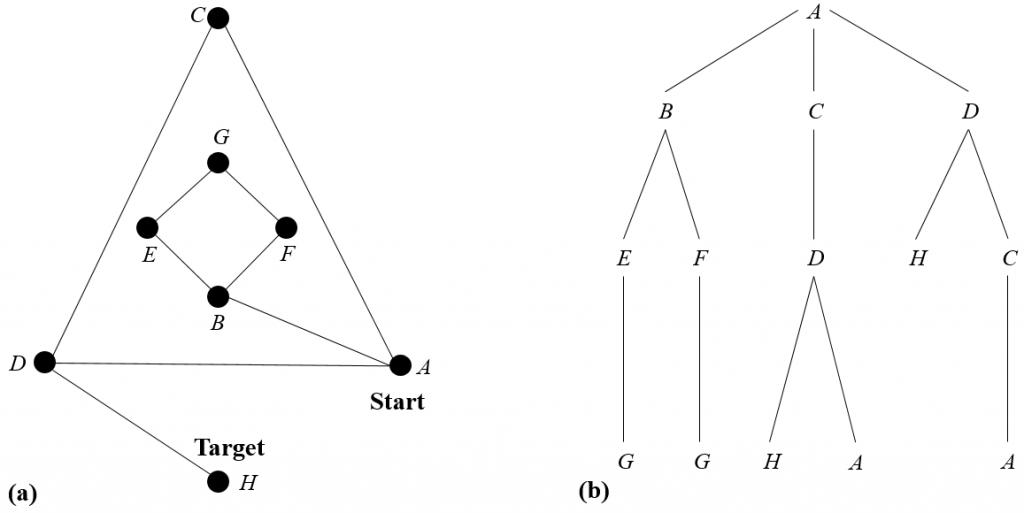
At times there is no graph representation available for the problem at the start of the process of finding a solution. In this case, whilst search is performed, a partial picture of the graph is gradually built up from nodes which have been explored. Here, for every iteration, all nodes adjacent to the one being explored according to set of transition rules are added to the graph (along with edges connecting them to the node being explored), this is called expanding the node. Practically, this is the application of all possible actions to that state. When doing this, it is important to keep track of nodes which have already been generated in the search. Here, every node must be explored at least once in order for it to be present. As a result of this, it is possible to sort the set of all nodes which have been reached into one set of nodes which have been expanded, and another set which have been added to the graph and not yet expanded. The rest of these is known as the open list or search frontier, and the second set is known as the closed list. The set of all paths from the node at which search began up to the set of open nodes gives the the search tree of problem, which gives an illustration of the part of the solution space which has been explored by the search algorithm at a given time. Possible search roots for up to three moves on the graph in figure (a) above are shown on the search tree for the solution of the problem in figure (b). There are multiple different methods for performing searches on graphs, one distinction between methods is the order in which the solution space is searched, this is commonly either breadth first or depth first which shall be discussed further here.
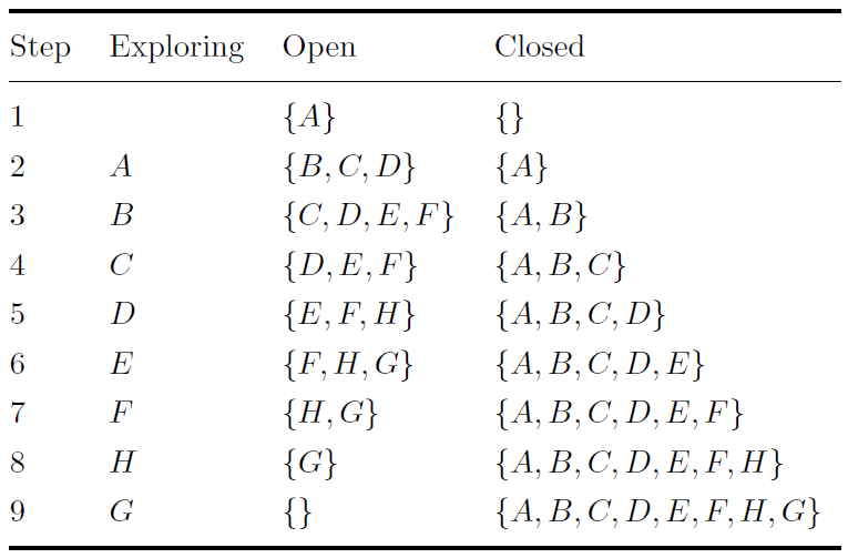
When performing breadth first search, the open set is considered to be a first in first out queue. So when a node is added to the open set, it is added to the bottom of the list. When a node is explored, the node at the top of the list is expanded and moved from the open set to the closed set. The result of this is that nodes are explored layer by layer and the graph is expanded from the start node. An illustration of this can be seen in the table to the left, which shows how the open and closed sets of nodes change as breadth first search is performed on the problem with the graph shown in figure (a).
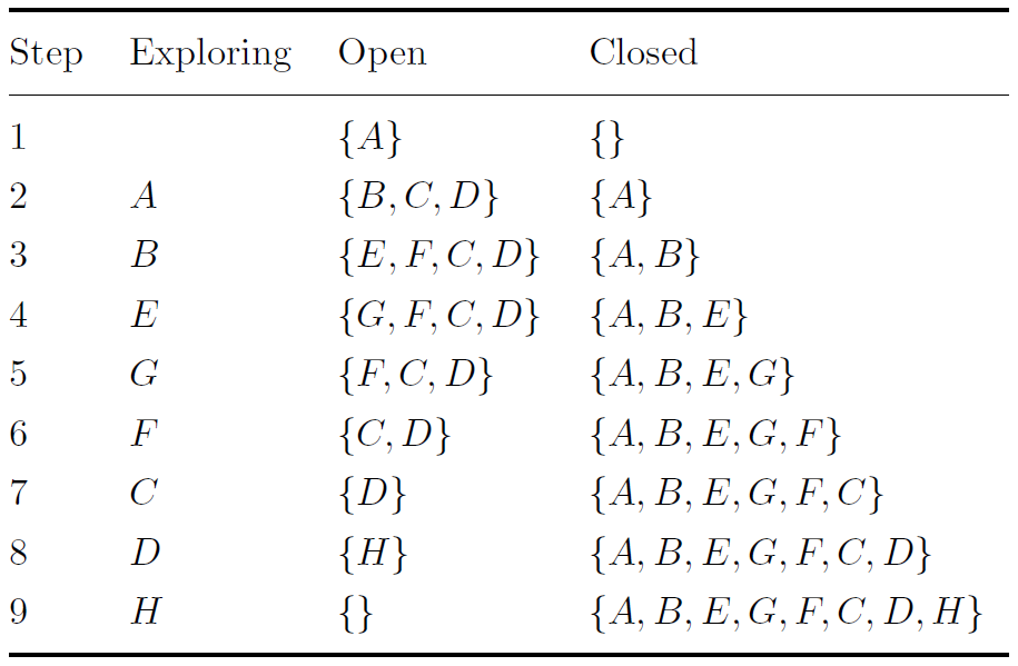
When performing depth first search, the open set is considered to be a last in first out queue. This means that when a node is added to the open set, it is added to the top of the list. It also means that when a node is explored, the node at the top of the list is expanded and moved from the open set to the closed set. The result of this is that every iteration generates a node connected to the last node expanded (unless there are none, in this situation the algorithm backtracks to the last node with an unexplored node adjacent to it). This means the search effectively explores a path until that path has been completely explored, then goes back to the point at which that path branches off and explores other paths from here, repeating this process until all paths have been explored. An illustration of this can be seen in the table to the right, which shows how the open and closed sets of nodes change as depth first search is performed on the problem with the graph shown in figure (a).
About the author