Networks and network data analysis have seen one of the largest growth in quantitative sciences recently. While their origins stem mostly from social connections, their applications are more wide spread. One particular example is creating a map of the brain and trying to capture connectivity of different parts of it. Therefore, we introduce networks here:
Graph Theory
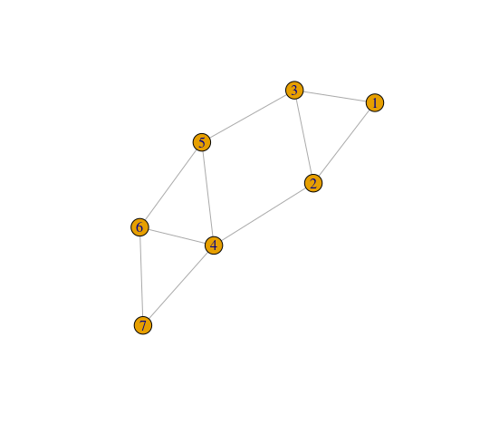
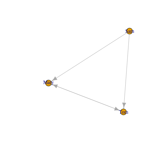
Networks are most easily represented in terms of graphs. A graph is a mathematical structure G(V,E), where V \subset \mathbb{N} is the set of vertices (also called nodes) and E is the set of edges. The graph is usually represented in a matrix form called: adjacency matrix. We illustrate this with a picture:


The left picture represents an undirected graph as there are no directions between the nodes and the right one, a directed one or digraph. For example Mary and Tom could be friends at work and share ideas between one another, but Sam might be just forwarding tasks and not participating in their evaluation at the end. While neural signals are directional, it can be shown that significant modelling can be achieved with undirected graphs, due to the undirected structure of the nervous system, see: article. In this case, the first row of the adjacency matrix of the left graph would be: (0,1,1,0,0,0,0), while the second row will take the form: (1,0,1,1,0,0,0), third:(1,1,0,0,1,0,0) and so on. By convention, self-connections are not allowed, hence zeros on the diagonals which correspond to the first, second and third vertices above. Can you see why the matrix will be symmetric?
So we saw how networks can be represented in a simple way. Why are they important in neuroscience? Well, neurons in the brain basically act as nodes and they are connected through structures called synapses, see figure below. The idea is that neurons, have a core (the circle), dendrites, which surround the core, an elongated body called an axon and nerve endings termed synapses. Basically, the axon serves the purpose of a wire with potential differences at the the two ends, hence electrical signals can travel through it. Once they reach the end of the axon, signals can transfer to the next neuron through connections established between the synapses of the first neuron and the dendrites of the second. Those connection can vary in strength, hence some neurons are better connected than others, leading to the notion of a weighted graph.

For the purposes of simplicity, we will not delve into weighted graphs now. What, however, seems particularly important is how brains have formed through evolution. Upon clinical trials, it has been shown that signals traveling through neurons share the following features:
- slow
- noisy
- energy consuming
This could be just biological properties that are hard to change. That is why the brain to some extent has evolved in such a way that electrical signals pass through a minimum number of neurons to reach their targets. That is not to say that the brain is trying to have as few neurons as possible, but is careful at how it positions them and forms the edges, so that a signal traveling from neuron i to j tries to follow the shortest path between them. For example, the shortest path between nodes 5 and 7 is of length 2 and can be achieved in two ways (i.e. going through nodes 4 or 6).
However, neurons do not only communicate between one another following the shortest paths. In fact, while shortest paths are preferable, a connection could be established though all paths, hence it makes sense to consider a set of k shortest paths. This leads to idea of a communication capacity. A simple way to assess the communication capacity C_{ij} between two nodes i,j, would be to find the weighted sum of all walks from the source node i to the destination node j. This will penalise the longer paths more, while shorter ones will have higher contribution. Hence:
C_{ij} = \sum_{n}\frac{\# \text{walks of length} \;n}{n!}.
Looking back at the left graph for nodes 5 and 7, we see that there are zero walks of size 1, hence the first term in the sum will be zero. Two walks of size 2, two walks of size 3 and so on. Therefore:
C_{ij} = 0 + 1 + \frac{1}{3} + \frac{1}{24} + \ldots.
However, computing this sum could be quite cumbersome for big graphs (remember brains have billions of neurons), so we need to find a simpler way of establishing this quantity. Looking back at the initial equation for the communication capacity, we see that in some sense (the factorial in the fraction) resembles the taylor expansion of e^{x}: \sum_{0}^{\infty}\frac{x^{n}}{n!}. Now, our toy model only has 7 nodes, but as graphs get bigger, the finite nature of the sum (partial sum) will converge to infinite one (as n gets bigger, the last terms become more negligible). But if this is true, then what should go in the power of the exponential?
Well, it needs to be something that contains the information about the edges of the graph, as we are interested in all walks of different lengths. To find the power component, let us look at the second power of a symmetric matrix. If M is a n \times n symmetric matrix, and noting that m_{ij} = m_{ji}, then:
M^{2}_{ij} = \sum_{k = 1}^{n}m_{ik}m_{kj} = \sum_{k = 0}^{n}m_{ik}m_{jk}.
Now, this basically means that instead of the usual row-column multiplication, we multiply the componentwise the i_{th} and j_{th} rows. Now, let us look at the first three rows of our adjacency matrix above. If we call our adjacency matrix A, then:
A^{2}_{13} = (0,1,1,0,0,0,0) \times (1,1,0,0,1,0,0) = 1.
So what does this mean? If we look at the graph, then we can see that there is only one connection between nodes 1 and 3 that is of size 2. So, essentially, we can find the number of connections of length n between the nodes i and j, by simply extracting the (i,j)_{th} component of the n_{th} power of the adjacency matrix. This also makes sense, because in our example, for node 1 to be connected to 3 via the link of length 2, we need both nodes to be connected to node 2, hence we should expect a non-negative contribution to the sum in the matrix product from the multiplication of the second entries. But this is exactly what we need in the computation of the communication capacity between two nodes. Hence, we can compactly express C_{ij} as:
C_{ij} = \sum_{n}\frac{\# \text{walks of length} \;n}{n!} \approx (e^{A})_{ij},\quad n\rightarrow \infty.
Fitting a network model
So great, we can now establish the communication capacity between different nodes. However, this involves the knowledge of the adjacency matrix, which could be very hard to obtain, especially if the inclusion invasive methods are needed. One way we can predict the edges for a given set of nodes is to fit a model to the nodes. The simplest one is known as the Erdos-Renyi Model.
The idea behind the Erdos-Renyi Model, is that for every pair of nodes (i,j), we can connect them with probability p. If we have n nodes, then the number of possible connections (edges) we can form would be \frac{n(n-1)}{2}, where we divide by 2 due to the undirected nature of the graphs we consider. Hence, the number of edges would follow a binomial distribution:
Edge\; number \sim Binomial\Big(\frac{n(n-1)}{2}, p\Big).
Therefore, we can extract the mean number of edges and the variance:
\mathbb{E}[Edge\; number] = p\frac{n(n-1)}{2}
Var[Edge\; number] = p(1-p)\frac{n(n-1)}{2}
Another notion that is useful in graph theory is the degree of a node, which represents the number of edges that are connected to it. In a graph with n nodes, for each node i there are n-1 possible connections to other nodes. Hence, its degree d_{i} would also follow a binomial distribution with mean and variance respectively:
d_{i} \sim Binomial(n-1, p)
\mathbb{E}[d_{i}] = p(n-1)
Var[d_{i}] = p(1-p)(n-1)
This information can help us construct the network and extract its adjacency matrix, hence establish the communication capacity between nodes. This can be particularly useful in catching early brain diseases, which could compromise some of the edges, hence change the communication capacity matrix. If upon discovery of unusual deviations from the normal communication capacities in a patient, early measures could be taken to prevent the progression of the disease.
Thank you for reading. I hope this post has encouraged you to explore further what networks are and how they can be used in practice, or how mathematics can be applied in medicine and help saving lives.