Markov Chains
Markov chains are a fairly common, and relatively simple, way to statistically model random processes. They have been used in many different domains, ranging from text generation to financial modeling. Overall, Markov Chains are conceptually quite intuitive, and are very accessible in that they can be implemented without the use of any advanced statistical or mathematical concepts. They are a great way to start learning about probabilistic modeling and data science techniques.
Weather example
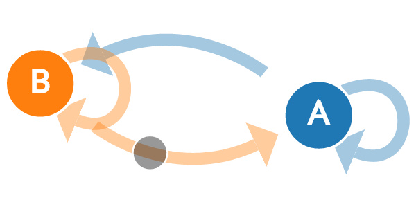
Imagine that when you wake up, you observe the if it is sunny or rainy each day. You might want to assign probabilities, such that given the state of the day today (sunny or rainy), what is the probability that tomorrow will be sunny? You can now use this distribution to predict weather for days to come, based on what the current weather state is at the time. This is schematically illustrated in the following picture:

Based on our observations, we have concluded the probabilities for those transitions above. In particular, if today is sunny, then we have 90% chance of remaining sunny tomorrow and 10% chance of raining. If, however, today is rainy, we have 50% chance of transitioning either to rainy or sunny day. Those transitions are also called jumps, and the system itself is termed: a Markov chain. The name, Markov, comes from the person, who invented them: Andrey Markov, a Russian mathematician. The feature that make them special is the so called memoryless property, which means that how the chain evolves only depend on the current state of the system. This is also the case for our weather model above, as whether it is sunny or rainy tomorrow depends only on what the state is now. This typically leaves them unable to successfully produce sequences in which some underlying trend would be expected to occur. For example, while a Markov chain may be able to mimic the writing style of an author based on word frequencies, it would be unable to produce text that contains deep meaning or thematic significance since these are developed over much longer sequences of text. They therefore lack the ability to produce context-dependent content since they cannot take into account the full chain of prior states.
A typical way to represent Markov chains is through their transition matrices, which contain information of how the move forwards in time. For our example above, the transition matrix will be of the form:
| 1: Sunny | 0.9 | 0.1 |
| 2: Rainy | 0.5 | 0.5 |
Hidden Markov Models
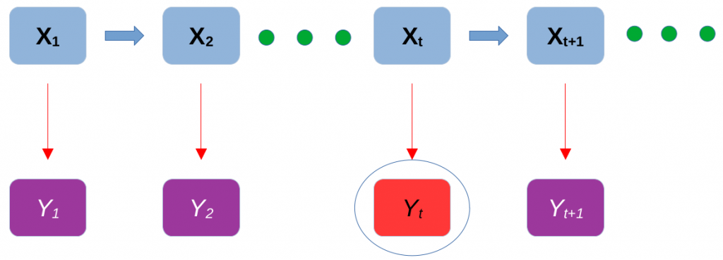
Before introducing the formal definition, let us first take a look at the following Figure:

Imagine that there is a process X that evolves in time. In this case, we will consider the so called jump chains, where each time step, 1, 2, . . ., will present a transition of the process on another stage. The process \mathbf{X} will be the unobservable component of the hidden Markov model and at each time, \mathbf{X}_{t} will contain information of possibly many unknowns that we cannot see. In our simple simulation example, \mathbf{X} will contain the number of rabbits R_{t} and number of foxes F_{t} at time t. Another assumption will be that if the process is currently at time t, how it evolves in the future will be independent of its past. Hence, this is the Markov process in the our hidden model.
Ok, so what can we see? Well, in practice we only observe noisy observations of some of the unknowns contained in the process \mathbf{X}. Furthermore, while in theory we could obtain observations at each transition, in practice it might not be possible. For example, you do not observe the population of rabbits each time they increase by one, but you might send a person to record their numbers once a month. This will be our noisy observation, say Y_{t} at time t. In our discussion, we will assume that some of the unknowns are unobservable even through noisy observations (this is realistic as we rarely see foxes). Additionally, we shall also assume that Y_{t} only depends on the current state of the system \mathbf{X}_{t} and not on the past. Mathematically, we can express a hidden Markov model as:
Definition: The pair (\mathbf{X}_{t}, Y_{t}) is a hidden Markov model if:
- \mathbf{X}_{t} is a Markov process, whose behaviour is not directly observable
- P (Y_{t} \in A|\mathbf{X}_{1} = \mathbf{x}_{1} , . . . , \mathbf{X}_{t} = \mathbf{x}_{t}) = P (Y_{t} \in A|\mathbf{X}_{t} = \mathbf{x}_{t}), for all t \geq 1 and any measurable set A
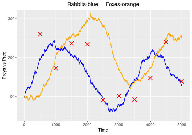
Simulation
If we assume that the individual variables in the hidden process \mathbf{X}, rabbits and foxes, follow a Poisson process, then, knowing the transition rates in the exponential distributions will determine how the process evolves. If we settle on a Gamma noise, where the mean of the Gamma represents the true state, we can simulate the system. The following plot represents the noisy observations as red crosses, foxes as the orange path and rabbits as the blue path:
