Remember our hidden Markov model for the rabbits and foxes from the previous blog? Well, let us recap quickly. It was a hidden Markov process, the state of which consisted of the number of rabbits and foxes at each integer time step, that we could not observe, but only had access to noisy observations of only the number of rabbits at some given times. Here we introduce some techniques that would help us approximate the hidden state of the rabbits.
Particle filters, also known as sequential Monte Carlo methods, are predominantly used to solve filtering problems arising in signal processing and Bayesian statistical inference. This means that the methods try to estimate a hidden Markov process (i.e. a process we do not actually see), based only on partial noisy observations. The term particle filters was first introduced in 1996 by Del Moral, [1], and was subsequently referred to as “sequential Monte Carlo” by Liu and Chen in 1998, [2]. This blog aims to introduce a number of filtering techniques, by starting from some simple methods and slowly improving them by establishing their weak points.
Background
The majority of research articles are devoted to the problem of filtering : characterising the distribution of the state of the hidden Markov model at the present time, given the information provided by all of the observations received up to that time. In a Bayesian setting, this problem can be formalized as the computation of the distribution p(\mathbf{X}_{t}|Y_{1:t}), i.e the distribution from which we can sample to estimate the hidden state at time t, given the observations. We can compute this distribution in a recursive fashion, using prediction and update steps. Imagine that you know p(\mathbf{X}_{t}|Y_{1:t-1}), which can be thought of prior for \mathbf{X}_{t} before receiving the most recent observation Y_{t}. In the prediction step, we can compute p(\mathbf{X}_{t}|Y_{1:t-1}) from the filtering distribution at time t-1:
p(\mathbf{X}_{t}|Y_{1:t-1}) = \int p(\mathbf{X}_{t}|\mathbf{X}_{t-1}) p(\mathbf{X}_{t-1}|Y_{1:t-1}) d\mathbf{X}_{t-1},
where the distribution p(\mathbf{X}_{t-1}|Y_{1:t-1}) is assumed to be known from the previous steps. In the following update step, this prior is updated with the new measurement using Bayes’ rule, which will become the posterior, before being used as the filtering distribution in the next update step:
p(\mathbf{X}_{t}|Y_{1:t}) \propto p(Y_{t}|\mathbf{X}_{t})p(\mathbf{X}_{t}|Y_{1:t-1}),
SIS algorithm and particle degeneracy
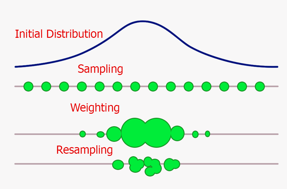
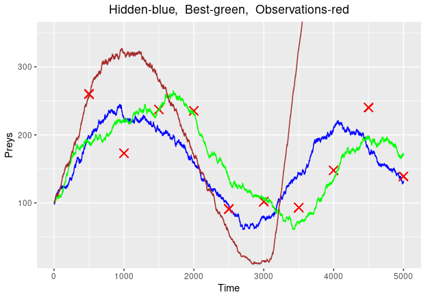
SIS stands for “sequential importance sampling”. The idea behind the SIS algorithm is to approximate the full posterior distribution at time t-1, p(\mathbf{X}_{0:t-1}|Y_{1:t-1}), with a weighted set of samples \{\mathbf{x}^{i}_{0:t-1}, w^{i}_{t-1}\}^{N}_{i=1}, also called particles. Then, the algorithm will recursively update the particle weights, to approximate the posterior distribution at the next steps. SIS is based on importance sampling, hence we need a proposal distribution. After running the algorithm for 10 observation points, we arrive at the following plot, where the green path is the best fit and the brown, the worst:
Since we used the weights to determine which path is the best one, we can plot how the weights change and in particular record the weights at the final observation:
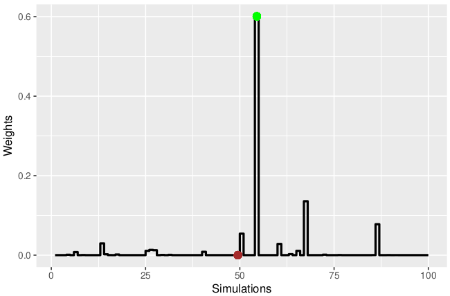
However, as we can see, the weight of the green path overshadows the others. In fact, if we add a few more observations, the weight of the green path will converge to 1. At this stage, we are wasting computational effort simulating the other paths, as since we are using the weights to determine the best representation of the hidden states, only the green path will be important. This is known as particle degeneracy. At this stage it is useful to introduce a quantity that tells us how many of our particles are significant.
Effective Sample Size
The effective sample size (ESS) is a measure of the efficiency of different Monte Carlo methods,such as Markov chain Monte Carlo (MCMC) and Importance Sampling (IS) techniques. ESS is theoretically defined as the equivalent number of independent samples generated directly formthe target distribution, which yields the same efficiency in the estimation obtained by the MCMCor IS algorithms. The most widely used and simple form of the ESS is:
\text{ESS}_{j} = \frac{1}{\sum_{i=1}^{N}(w_{j}^{i})^{2}},
where w_{j}^{i} is the normalised weight for the i^{th} particle at time observation j. This is intuitive, as if each of the particles have weights 1/N, where N is the number of simulated particles, the ESS will also be N. Therefore it is a measure of how many of our particles are properly exploring the space around the observations. We expect the ESS to deteriorate with the number of observations increasing as essentially we collapse onto one “important” particle with a weight almost 1. Upon plotting the ESS for 10 observation, we get:
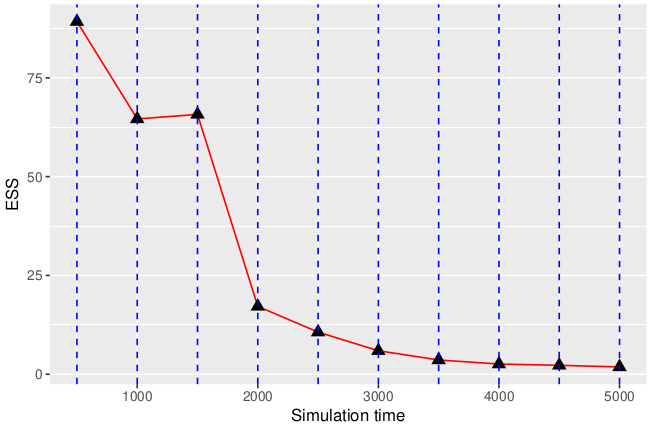
As we can see, the ESS starts from a value close to a 100, (91.8 in our case). In our simulation we used 100 particles, so on the first observation, quite a lot of them are representative of the hidden state, hence we can continue to simulate them. However, after the 3^{rd} observation, the ESS quickly drops to zero, meaning that we have achieved particle degeneracy. One solution could be to resample the particles at each observation from a multinomial distribution.