Ambit Stochastics: How to Model Spatio-Temporal Fluctuations

During the second term of the Masters year at STOR-i, we are introduced to 4 different active research areas by the experts researching in what are known as the Masterclasses. With a focus on one area per week for four weeks in a row, we are given talks by and engage in interactive activities with a researcher in that area. A few months after this we then pick two of the topics, and in groups and pairs respectively, create a poster on one, and give a presentation on the other. This gives the Master’s students our first go at making an academic poster, a somewhat tricky task that must balance technical accuracy, graphic design, and intrigue. Such posters are widely used at conferences to give researchers from outside your area an idea of what you’ve been working on, how it works, and how it can be used in the real world.

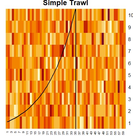
The masterclass I’d like to discuss in this post was an introduction to the field of Ambit Stochastics, given by Almut Veraart of Imperial College London. Before we can even discuss that, we must first introduce spatio-temporal processes. As you might expect, these are statistical model which seek to describe how things change as they move around in space, and as they progress through time. A very common example of this is temperature. If we had an array of thermometers spread across a landscape, they would all give slightly different readings at the same time, due to the natural spatial fluctuations of temperature. These readings would also change as time progresses in a variety of different ways. Day to day, these readings will fluctuate according to the day-night cycle, warmest at midday, and coldest as night. Over a year, these measurements will change according to the seasons. Over a longer period of time, we may also see a general upwards trend due to climate change. On top of all of this, we will also see smaller, noisier, more complicated fluctuations. Along these lines, spatio-temporal processes can be split up into two parts: deterministic overall trend, and random noise. The goal of Ambit Stochastics is to model the noise component, and come to better understand the complicated fluctuations that cannot be properly modelled in the overall trend. Below is the (admittedly scary looking) formulation of the overall model, which we’ll follow with a piece-by-piece breakdown.

\(Y_t(x)\) describes the thing we’re trying to model (say, temperature) at a time \(t\) and spatial position \(x\). \(\mu\) would simply be our trend term. The big ugly integral is actually a stochastic integral, where everything under the integrand is being integrated against an underlying source of spatio-temporal randomness given by \(L\). As a technicality, this is a Lévy basis, and can be considered a generalisation of a Brownian Motion, which may be a much more familiar random process for some. The set \(A_t(x)\) gives the set of spatio-temporal points that are thought to have any impact on \(Y_t(x)\). For example, this may potentially include all spatial information, but only from all the times \(s\) before \(t\). The main function \(g\) is called the kernel, and intuitively describes a weighting of points \((\eta,s) \in A_t(x)\) in terms of how much they impact \(Y_t(x)\). Something we might expect \(g\) to do is decrease for points further away from \((x,t)\) in time and space, as these would be expected to have less of an impact. Finally, we have the stochastic volatility term \(\sigma_s(\eta)\), which describes the intensity of the random fluctuations at a given spatio-temporal point.

It’s worth giving an example to explain what’s going on. Here we have a heatmap displaying ten samples of randomness for each off the times from 1 to 60 in one unit intervals. For simplicity, we don’t consider a spatial component here. This is a visual representation of collecting all the randomness which affects a process \(Y\) at time 35.5. Here, our ambit set is displayed as [1,35.5], but could theoretically stretch back to \(-\infty\). The area under the exponential curve represents all the randomness being collected. Clearly, nothing from the future is being collected. We also see that, as we move back through time, less and less of the randomness is being taken into consideration, allowing more recent information to have a greater impact. As time progresses, we would shift the curve rightwards, providing the most weight to the more recent information, and less weight to old information.

We can see that the above formulation provides a very flexible model for modelling the random nature of a spatio-temporal process, as we are able to choose different ambit sets, kernels, volatilities, and underlying Lévy bases. Now that we have a basic understanding of these models, we can discuss how they can actually be used for real world problems, as described by Veraart during her masterclass presentation.

In fact, we can tie this post back to my very first post, as the application combines with Extreme Value Theory! Our specific example wishes to model extreme rainfall at Heathrow over time. We do this using the threshold model, defining the threshold to be the 95% quantile of the data. Standard inference techniques (also introduced in a previous blog) don’t quite work here, as such techniques rely on independent data. That is to say, if we were to use such techniques, we would be assuming that rainfall on one day doesn’t affect rainfall on another day. This isn’t true! Rainfall (or therefore lack of) one day can absolutely affect the chances of rainfall the next day. Therefore, we must be able to model this dependence structure, which we can do using Ambit Stochastics. The aspect we model this way is the probability at a certain time of exceeding our threshold, allowing the model to dynamically incorporate the history of the rainfall into probability of exceedance, rather than using a flat constant 5%. This allows the dependence structure of the rainfall data to be more accurately modelled, which in turn allows us to achieve better estimates of the GPD distribution that models the exceedances of the threshold. This strategy of having multiple layers of uncertainty to estimate, both the probability of exceedance and the distribution of those exceedances, is known as hierarchical modelling, which can better represent how uncertainty can cascade through a model’s estimates.

Ambit Stochastics have had a wide range of other applications too, including the modelling of financial markets, tumour growth, designing wind farms, and plenty more. For simplicity’s sake, I’ve left out a lot of technical details here, as this is just a surface level taste of what can be done with this approach to spatio-temporal modelling. If you’re interested in diving further into this area, Veraart co-authored the textbook “Ambit Stochastics” (2018) with  Ole E. Barndorff-Nielsen and Fred Espen Benth, which gives a comprehensive and in-depth overview of the field to date.