Can a Computer teach itself? A Look at Machine Learning

As mentioned in an earlier post, during the MRes year at STOR-i we write papers on two “Research Topics”, one which is seven pages long, and one which is a more substantial twenty pages. Feedback from my first Research Topic paper raised a few issues about my writing style, so the second paper gave me an opportunity to refine my style, and make something a lot more exciting and readable. Something that very much helped with this was the choice of an interesting topic known as Reinforcement Learning. However, Reinforcement Learning is a category of something that I looked into for my EPQ during my A-Levels, which I’d like to discuss in this post (and see how much I remember). So, in this post, I’m going to talk about Machine Learning.

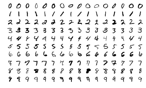
Machine Learning, or ML, is an area in both mathematics and computer science whose goal is to find ways in which a computer could teach itself to perform a task. This is in contrast to the traditional way to make a computer perform some task, which generally involves explicitly writing an algorithm or program. However, for tasks with a great deal of nuance, this becomes extremely difficult, so we turn to ML to solve the problem for us. A well-known example is image classification, where we want a computer to be able to look at a picture of something and say what it is. A famous starting point is the recognition of hand-drawn digits: we want to give a computer a picture of some number, and for the computer to correctly identify that number. How do we even begin to do something like this? The approach we’ll describe here has two components: a LOT of data (an example of which is the MNIST dataset), and Neural Networks.

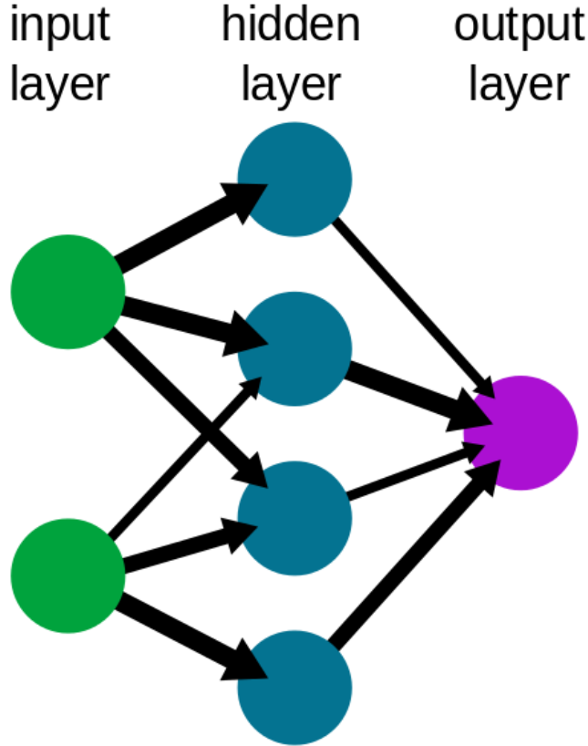
Neural Networks, or NNs, are a family of relatively simple but powerful models which are based on the structure of the brain. We start with an input layer, which is simply where all of our information goes in. Each little bit of information is stored in a node; for example, in a black and white digit image like the ones above, each pixel of the image would have its own node. This then feeds into a hidden layer of nodes, where each node takes in some of the information from the input layer. However, each node doesn’t look at all the information equally. Look at the second blue node on the left, it has a thick arrow from the top input, and a thin arrow from the bottom input. This represents how the inputs are weighted, meaning the second blue node considers the top input more important than the bottom. This is done by a simple linear combination; if we call the inputs \(a\) and \(b\) and the respective weights \(w_1,w_2\), then the node receives \(w_1a+w_2b\). This then goes through some “activation function” \(\sigma\) to slightly manipulate the result. This is done with all nodes, all of which have different weightings, allowing the layer to deduce certain “features” of the input. The output layer then does much of the the same, but treat the hidden layers as inputs. Despite the image, output layers can have multiple nodes like any other layer. For example, for digit recognition, it could have ten output nodes, all of which give a probability that the input is a certain digit. This allows the network to then express uncertainty, and doesn’t force it to give a solid answer. Neural Networks can then be extended to have multiple layers with loads of weighted connections and nodes, and these more complicated NNs are known as Deep Neural Networks.

Now that we have a model, how do we make it correctly recognise images? The specific type of machine learning we’ll use is known as supervised learning. All of the hand-drawn digits in the MNIST dataset actually come with a label stating which digit it represents. Then, by comparing the output of the neural net to the actual answer, we can come up with a measure of how wrong it is. The most common measure is Mean Squared Error, or MSE. Call our image input as a vector \(\mathbf{x}\), our neural net a function \(f\) which outputs a length-10 vector of probabilities, and the length-10 vector containing a 1 in the position of the actual known label and 0s elsewhere \(\mathbf{y}\). The MSE of this one datapoint is then \(\frac{1}{10}\sum_{j=1}^{10}(f(x_j)-y_j)^2\), where the \(j\)s index the components of the vector. We then sum this up for every image in the dataset, giving a measure of overall error which we call the cost function, \(C\). As \(C\) depends on the weights \(\mathbf{w}\) of the neural net, we can write this as a function \(C(\mathbf{w})\).

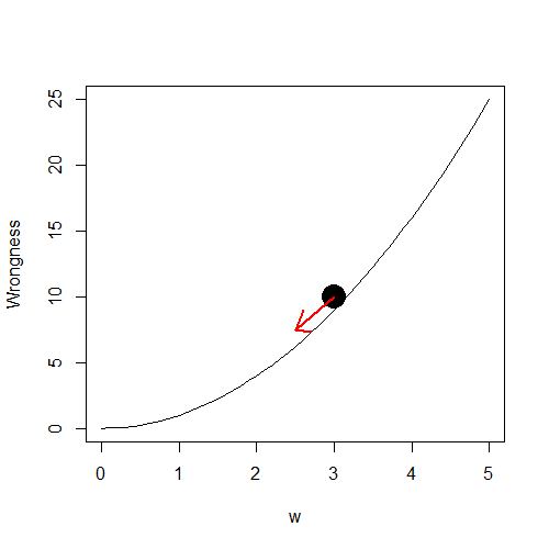
Now that we have a measure of “wrongness”, our task is now to make the neural net less wrong. We do this by repeatedly having the weights of the neural network take small steps in the direction that make it less wrong. This is often known as Gradient Descent, and can be explained as working your way down a foggy mountain by always taking small steps down the the steepest slope. The lower down the “mountain” we get, the less wrong we are. This can be represented by the update

\(\mathbf{w}\gets \mathbf{w}\,-\,\alpha \nabla_{\mathbf{w}}C(\mathbf{w})\)

where the \(\nabla\) represents the gradient, or slope, of whatever it’s applied to, and \(\alpha\) represents the “step-size”. Doing this repeatedly for a long time allows our neural net to keep getting less wrong, until it is the least wrong it can be. The mathematically inclined reader might recognise the process of finding the gradient as differentiation (skip this part if this is new to you), which is exactly what we’re doing! This is why we need to have a differentiable cost function such as squared error, but it also means the neural net itself must also be differentiable with respect to the weight values. Luckily, it is! This is basically done by chain-ruling each layer of the network, and using differentiable activation functions at each node. Its messy, but thankfully smart neural net people have written code to do that for us.

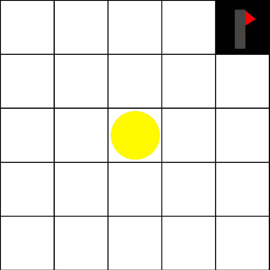
This supervised learning approach provides a framework to solve the problem of giving the correct output for a given input, based on an abundance of data. We can say that the network makes a single decision. However, we can consider tasks where we have to make multiple decisions sequentially, where each decision affects the state of the problem. An example of such a problem is given by video games, where each decision (the buttons pressed on the control) affects the state of the game (whatever’s shown on the screen). So how might a computer learn to solve such a task? The supervised learning approach would be to give a neural network an abundance of data which pairs states with their optimal action, however we have a better source of data: the game itself! We can instead find an approach might learns through trial and error by interacting with the environment, and this is known as Reinforcement Learning!

A nice and simple introductory example for Reinforcement Learning, or RL, is known as the Gridworld. The Gridworld has simple rules: you can move up, down, left and right; you are penalised for falling off the grid, you are slightly penalised for taking too many steps, you are rewarded for “collecting” certain items, and the problem ends when you reach the goal. You can start at any position on the grid, but if you fall off, you always return to the bottom-left. The task of RL in this case is to maximise told reward, which is understood in context as collecting the coin and reaching the goal in a minimum number of steps. However, while this is intuitive to us as humans, the computer starts by knowing nothing about the problem; it doesn’t even know what up, down, left and right are. So, how does it learn? We follow an approach known as Generalised Policy Iteration, or GPI. By “policy”, we mean the rule for which action we take for each state. We start off with a completely random policy, which moves in any direction for any state, where the state is simply comprised of the position of an agent and whether or not the coin has been taken. We then store an estimate of how good we think the policy is by storing an estimate of long term reward in a function \(Q(s,a)\), where \(s\) and \(a\) are the state and action. GPI works by repeated improving estimates of how well the policy works when using certain actions, and then improving the policy by assigning more probability to the actions thought to be better.

So how do we evaluate this random policy, or improve our estimates? When we take each random action \(a\) in a state \(s\), we observe a one-step reward \(r\) and end up in a new state \(s’\). Then, $r + Q(s’,a’)$ gives an improved, or “less wrong”, estimate of \(Q(s,a)\), as we include new information about the reward received and the state we end up in. We then use the update \(Q(s,a) \gets Q(s,a) + \alpha(r + Q(s’,a’) – Q(s,a)).\) Much like how we trained the neural net, we update these \(Q\) values by taking small steps determined by \(\alpha\) in the direction thought to make them less wrong. In the context of RL, this is known as temporal difference learning. You might wonder where this \(a’\) term comes from, and there are two choices for this. It’s either the next random action taken by the policy, or the action currently thought to be the best action for state \(s’\). These two approaches are called SARSA and Q-Learning, respectively. Based on this improved estimate of performance, we then update the random policy itself by assigning more probability to the actions which are thought to be better. Over time, this makes the policy less and less random and we assign more and more probability to the best action, until the probability of picking the best action in any state approaches 1.

In this post, I’ve introduced two types of Machine Learning: supervised learning and reinforcement learning. However, I’ve only introduced RL for a very simple problem where each \(Q\) value can be stored for each pair of states and actions. However, most problems are far more complicated, and the number of possible states is massive! Consider even an older video games like Super Mario Bros; the number of possible frames is seemingly endless! The trick here is to combine RL with neurals nets to obtain Deep Reinforcement Learning. Simply put, rather than storing each \(Q(s,a)\) value explicitly, we represent it through a neural net with \(s\) and \(a\) as the input layer. When we do updates, we simply combine the way we do neural net updates (shifting weights around) with the way we do \(Q\) updates. This then allows RL to tackle far larger problems and achieved far more impressive feats, even playing Chess to a grandmaster level like AlphaZero. It is these kind of modern achievements which make Machine Learning a very exciting and modern field.