
If you ever took a programming module where you had to build an algorithm to compute something, you were most probably asked about its complexity. Well, if not, it’s a good practice to check if the algorithm you wrote is efficient. No one wants to have the programme running for hours if there are faster options to achieve similar results, am I right? A common way to evaluate the complexity of a model is using Big \mathcal{O} notation. But what is it?
Big \mathcal{O} notation is a mathematical property used to describe the asymptotic behaviour of functions. It gives us information about how fast a function grows or declines. It has many applications and one of them is to analyse the cost of algorithms.
If you are familiar with this notation applied to programming, you may know that the most common complexities are:
- \mathcal{O}(1)
- \mathcal{O}(\log(n))
- \mathcal{O}(n)
- \mathcal{O}(n\log(n))
- \mathcal{O}(n^2)
We can also have \mathcal{O}(2^n) and \mathcal{O}(n!) , but these are not that common. Okay, so I have already listed the most frequent complexities, but how can we see which one is our algorithm?
\mathcal{O}(1)
This seems the better one, right? Well, it is. In fact, independently of the input data size, say n , the algorithm will take the same time running. So, for example, if the goal of your algorithm is simply to assess an element of an array, or just adding one element to a fixed size list, then it won’t depend on n. Getting this complexity is the best you can aim for. Although, of course, in some cases (most of the cases, really), you won’t be able to get it.
\mathcal{O}(\log(n))
If your algorithm runs in a time proportional to the logarithm of the input data size, that is \log(n) , then you have \mathcal{O}(\log(n)) complexity. This type of complexity is usually present in algorithms that somehow divide the input size. One example is the Binary search technique:
- Assume that the data is already sorted. This method starts by selecting the median, say med , and then compares this value with a target value (chosen a priori), say y . It then has 3 options:
- If med = y, then there was a success
- If med > y, then it finds the median of the upper half of the data and compares it again with y
- If med < y, then it searches for the median of the lower half of the data and performs the same comparison
- The algorithm stops when med = y or until it’s impossible to split the data.
\mathcal{O}(n)
This one is as straightforward as the \mathcal{O}(1). If the time taken to perform the algorithm grows linearly with the n, then the complexity is of \mathcal{O}(n). An example of an algorithm with this complexity is if we have a list and we want to search for its maximum. It will iterate over the n elements of the list, storing the maximum found at each step.
\mathcal{O}(n\log(n))
As in the \mathcal{O}(\log(n)), this complexity is typical of algorithms which divide the input data set. One example is the Merge sort technique: briefly, it first divides a list into equal halves and then combines them in a sorted way. Consider a list of 4 unsorted elements, for example \{3, 1, 2, 5\} . First, the data will be split into two lists of 2 elements, that is \{3, 1\} and \{2, 5\} and then these two lists will be divided into 4 lists of 1 element each, that is \{3\}, \{1\}, \{2\} and \{5\} . In the next step, the algorithm will sort the elements by the 4 last lists and combine them into two lists, that is \{1, 3\} and \{2, 5\} . The final step is to combine these two lists into one sorted, that is \{1, 2, 3, 5\} .
\mathcal{O}(n^2)
The last complexity I’m going to talk about is the \mathcal{O}(n^2) . As you may have guessed based on the previous ones, this will happen if the algorithm runs in a time proportional to the square of the size of the input data set. This may happen if you have, for example, two nested loops iterating over n^2.
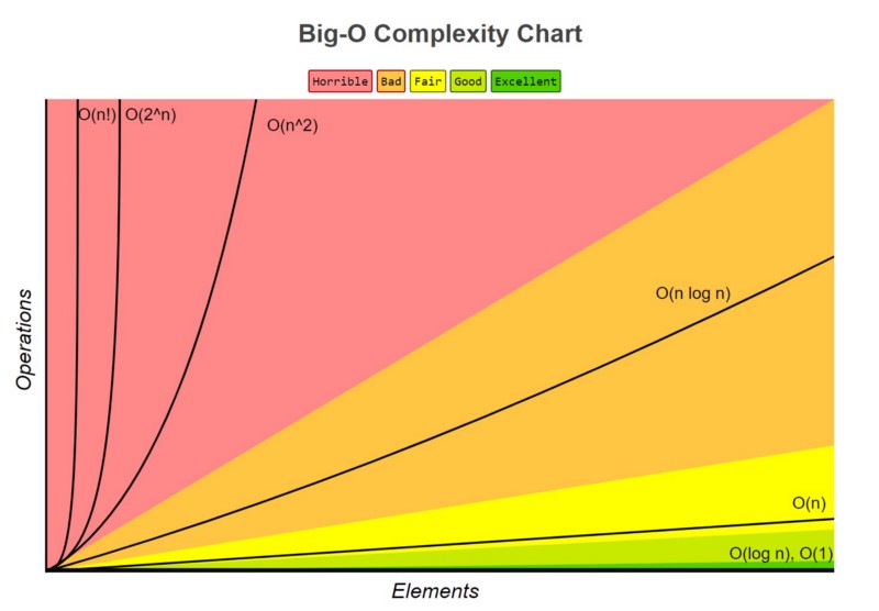
These are not the only possibilities, but they are the most common to happen. You can have complexity of \mathcal{O}(n^3) if instead of two nested for loops, you have three, and so on. A very good way to evaluate the performance of your algorithm is by plotting the time it takes to run and then compare its shape with these common complexities. The following graph may be useful for that.
I hope you find this post interesting and useful. You can see more here:
- https://www.bigocheatsheet.com/
- https://rob-bell.net/2009/06/a-beginners-guide-to-big-o-notation
- https://www.freecodecamp.org/news/big-o-notation-why-it-matters-and-why-it-doesnt-1674cfa8a23c/
- https://stackoverflow.com/questions/11032015/how-to-find-time-complexity-of-an-algorithm
Hope to see you soon!