Traditional statistics usually involves the breakdown and analysis of the general behaviour of a set data, with the aim being to gain insight into the average behaviour of a system, which events or results that are most likely to occur and to what degree do events vary. It is not uncommon, however, to encounter scenarios where the long run average value is of little concern to the analyst. Rather, it is the potential impact of the most extreme results of the series that are of critical importance (for example the average water height of a river may be of little concern when evaluating the effectiveness of flood defences, but the highest water levels pose a significant threat to people and industry nearby). Welcome to an introduction into the fundamentals of extreme value analysis.
The first issue is asking yourself “What actually is an Extreme Value?”. Clearly an Extreme Value is large, but how do you define one?
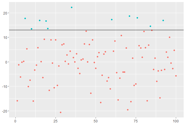
Generally, there are two methods to choose from when defining what an extreme value is. The first is to define an extreme value as the greatest value observed per naturally occuring block of data over the dataset. The second is to define some value \(k\), possibly some very high quantile, and designate any observation \((X_i > k)\) as an extreme value in the sequence. The benefit of the latter method is that we naturally obtain some form of block structure within the extremes which one find useful to analyse, although it is accompanied by its own set of difficulties.
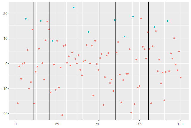
If the data has a clearly defined structure (eg: year sized blocks), then we look to option one with the aim to fit a Generalised Extreme Value (G.E.V) distribution to the extreme data.
If there exists sequences of constants \(\{a_n > 0\}\) \; and \; \(\{b_n\}\) such that
\begin{equation} \label{M_n^*}
\mathcal{P}\{M_n^* \leq z\} = \mathcal{P}\left\{\frac{M_n – b_n}{a_n} \leq z \right\} \rightarrow G(z), \;\; as \; n \rightarrow \infty
\end{equation}
then \(G(z)\) belongs to one of three extreme value distributions regardless of the unknown distribution of \(F\). Namely the Gumbel, Fr\’echet or Weibull distributions, each have varying behaviours but can be generalised into a single family. The (G.E.V) family, location parameter \(\mu\), scale parameter \(\sigma\) and shape parameter \(\xi\) is given by
\begin{equation} \label{GEV}
G(z) = \exp\left\{ -\left[ 1 + \xi\left(\frac{z – \mu}{\sigma}\right)\right]^{-\frac{1}{\xi}} \right\},
\end{equation}
with the requirements that \((\sigma > 0), (-\infty < \mu < \infty) and (-\infty < \xi < \infty)\), with \(\xi\) determining which of the three models the G.E.V fits.
If instead, we define any event \(X_i\) as an extremal if it exceeds some large threshold \(k\), it is natural to consider how much larger an event is over this threshold \(k + y\) and how likely that event is to occur. This can be modelled for the unknown distribution \(F\) by rearranging to
\begin{equation*}
\mathcal{P}\{X > k+y \;|\; X > k \} = \frac{1 – F(k+y)}{1 – F(k)}, \;\; for \; y>0.
\end{equation*}
The general family for threshold maxima is the Generalised Pareto (G.P) family of distributions. Fundamentally, there exists a relationship between the G.E.V and this new family. For a given sequence, if for an imaginary block structure there exists a suitable G.E.V model for the threshhold data, then \(G(z)\) is a member of the G.E.V family where it is possible to show that for a large enough threshold \(k\),
\begin{align*}
\mathcal{P}\{X<k+y\;|\;X > k \} = H(y) = 1 – \left(1 + \frac{\xi y}{\sigma + \xi(k-\mu)}\right)^{-\frac{1}{\xi}} \\ \Rightarrow \;
\mathcal{P}\{X>k+y\;|\;X > k \} = \left(1 + \frac{\xi y}{\sigma + \xi(k-\mu)}\right)^{-\frac{1}{\xi}} \;,
\end{align*}
for values of \(y\) such that \(y>0 \; , \; \left(1 + \frac{\xi y}{\sigma + \xi(k-\mu)}\right) >0 \). Hence, if, for block maxima, the sequence can be shown to have a suitable approximation to the G.E.V family, then there exists an approximate G.P family for modelling the threshold maxima with the same \(\xi\) value as the corresponding G.E.V distribution. Moreover, the construction of the G.P distribution is irrespective of the choice of block size for the G.E.V distribution, as long as the block sizes are large enough.
Further, it is possible to rearrange the probability into a more useful form to calculate the return levels which, for the marginal distribution of some value above the threshold \(\mathcal{P}\{X>x\}\;,\;x=k+y\) is given by
\begin{gather} \label{GPzettas}
\mathcal{P}\{X>x\} = \mathcal{P}\{X>k\}\left(1 + \frac{\xi (x-k)}{\sigma + \xi(k-\mu)}\right)^{-\frac{1}{\xi}} \\ = \zeta_k\left(1 + \frac{\xi (x-k)}{\sigma + \xi(k-\mu)}\right)^{-\frac{1}{\xi}}
\end{gather}
This is the form of the return level equation, where the solution \(x=x_p\) is the level that is exceeded, on average, every \(p\) observations such that
\begin{equation*}
\zeta_k\left(1 + \frac{\xi (x-k)}{\sigma + \xi(k-\mu)}\right)^{-\frac{1}{\xi}} = \frac{1}{p}.
\end{equation*}
This is particular useful for anticipating what maximum level is likely to occur over a given period of time. For example, if we need to build flood defenses to protect against floods that occur on average every 100 years, we can set \(x=x_p\) as the time length and solve for the hight required, assuming the model is a suitable fit.
Once a model is chosen, and many parameters can be tested to find the best fitting option available, one can perform inference via likelihoods to obtain confidence intervals and estimates as needed numerically.
This was only a brief introduction. The literature is deep and there are many applications beyond these simple examples. One also needs to consider the suitability of a selected model, any dependence in the data and what information is of critical importance.
Given the sheer amount of examples one can easily imagine where extreme values are the dominant issue, I think it is clear how applicable to study is. Hopefully this introduction provided you with a small insight into that world. All the best,
– Jordan J Hood