Computers aren’t getting faster anymore. Well, computers are still getting “faster” but not in the traditional sense. The speed of computers
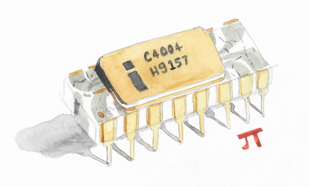
was historically given in terms of the clock speed or frequency of the Central Processing Unit (CPU). After the introduction of the first commercial CPU in 1971 (The intel C4004 that I’ve attempted to capture the likeliness of above), the frequency of CPUs was increasing linearly in time until the early 2000s when the frequency of CPUs began to plateau. The reason for this is one of power efficiency and heat output. The heat output of CPU transistors increases with frequency and above a certain frequency it will become too much for the CPU to operate at safe temperatures (i.e. not melt).
This issue meant that around 2004, semiconductor manufacturers decided to shift their CPU design philosophy from trying to increase clock speed to increasing the number of CPU cores on each chip. This had the effect of increasing the computational power of CPUs whilst maintaining safe temperatures. Heat is dissipated better from the multiple CPU cores running at moderate frequencies. Another advantage of multiple CPU cores are that they are capable of running separate streams of instructions to each other which is the basis for parallel computing.
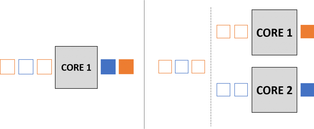
The previous focus on clock speed of a single core CPU, plus the fact that it is generally easier, meant that historically the algorithms used in computer programming were based on serial execution in which the instructions in the algorithm are executed by the CPU one after another in a sequence. This is illustrated on the left had side of the figure below where the tasks “enter” and are processed one by one. The increasing prevalence of parallel computing hardware such as multicore processors and clusters of linked multicore processors has given rise to a new way of approaching algorithm design. If it is possible to design an algorithm such that certain instructions\tasks can be computed simultaneously, then these tasks can be computed in parallel by several CPU cores (as illustrated on the left of the figure) to achieve a speed-up in the running time of the algorithm.

This often runs into a few challenges. For example, many of the serial algorithms that have been developed to perform certain computational tasks that are dependent on the outcome of other tasks. This means that dependent tasks often cannot be executed in parallel. An algorithm that consists of many dependent tasks will be difficult to redesign in a way that will benefit from parallelisation. Another challenge that is encountered is that new errors arise due to parallelisation. For example, the designer of a parallel algorithm has to be very careful that parallel tasks that work on the same data do not influence how that data appears in other tasks such that the result varies depending on which task is completed first.
Despite this, it is often worthwhile to try and overcome these challenges because of the resulting increase in speed of the algorithm. It’s likely to not just an immediate speed-up either as parallel algorithms will continue to increase in speed as more parallel cores become available.
A simple example of an algorithm that can be sped up using parallelisation is an algorithm designed to sort a list. Consider splitting the list up into \( N \) smaller lists, where \( N \) is the number of available parallel cores, and then sorting those smaller lists in parallel. These sorted lists can then be joined back together and the joined list can be sorted easily as it is just a list of sorted blocks. Sorting the list in this manner results in a speedup for lists of an appreciable size.
Another example that is more relevant to statistics and OR is Monte-Carlo sampling (Check out STOR-i student Hamish’s 60 second stats post on Monte-Carlo for a review on how Monte-Carlo sampling works). Consider the simple example of approximating \( \pi \) using Monte-Carlo sampling. We typically do this by sampling randomly within a square that encloses a circle, such as the one shown below, and labelling points based on whether they fall into the circle or not. We can then approximately calculate \( \pi \) by using the ratio of points that fall into the circle and those that don’t. Consider splitting the square into four quarters. It would then be possible to perform Monte-Carlo sampling on each of these quarters on four parallel cores and then using all four ratios obtained to calculate \( \pi \) . In this manner, we can perform more samples in the same amount of time, increasing the accuracy of the approximation.

In general, parallelisation has the potential to speed up many of the algorithms that are essential in computational statistics and operational research such as the particle filter or branch and bound methods for solving integer programs. In many of these cases, parallelisation requires the implementation of intelligent mathematical solutions to try and overcome some of the dependency problems I discussed earlier.
Relevant Links
Paper on the parallelisation of advanced Monte Carlo methods


This blog site is extremely cool. How can I make one like this ?