K-Means Clustering

In my previous blog, I introduced Supervised and Unsupervised learning methods. We will learn about one of the unsupervised learning methods called Clustering in this blog.

Clustering involves dividing a population or set of data points into groups so that the data points in the same group are more similar than those in other groups. The goal is to group similar traits into clusters and assign them to groups. There are several approaches to the task of clustering:

• Hierarchical clustering (agglomerative, divisive) – Define a set of nested clusters organized as a tree.
• Model-based clustering (mixture models) – A statistical modelling framework based on probability distributions.
• Partitional clustering (K-means, K-medoids): Division of the set of data points into non-overlapping subsets (the clusters) such that each data point is in exactly one subset.

In this blog post, we will focus on K-means clustering.

What is K-Means Clustering?

The K-means clustering algorithm depends on two parameters, the number of clusters and Cluster centroids. For a particular choice of the number of clusters K, the objective is to minimize the squared distance of the points within each cluster from its center (Referred to as a centroid). The algorithm is initialized by randomly picking the centers of each cluster and then assigning each data point to the closest centroid. After all the data points have been assigned to clusters, the centroids are updated to be the mean of all the data points for each cluster. Having updated the centroid values, we can assign each data point to its closest updated centroid, and then recompute the centroid values. The process is repeated until the centroid positions stop changing between K clusters. For a more detailed understanding, please check this blog.

How to determine what value to use for K?

The number of clusters are unknown in most cases. In such cases, measures of internal validation like, Calinski – Harabasz index and Silhouette can be useful to select the number of clusters.

Calinski – Harabasz index

The K-means algorithm returns the clustering minimizing within the sum of squares (WSS). The WSS measures the variability “within”, that is the variability between the data points assigned to cluster K and the corresponding centroid. The between clusters sum of squares (BSS), measures the variability “between”, that is the variability between the clusters accounting for the center of the data. Because the total variation in the data, the total sum of squares (TSS) is fixed, minimization of WSS corresponds to the maximization of BSS. The Calinski-Harabasz index is given by:

CH = \frac{\frac{BSS}{(K − 1)}}{\frac{WSS}{N-K}} with CH = 0 when K = 1

The Calinski-Harabasz index compares the relative magnitudes of BSS and WSS, accounting for K and N.
A large value of this index for a given value of K is an indication of a clustering solution with low within variability and large between cluster variability.

Silhouette

The silhouette is a measure of how close each point in one cluster is to points in the neighboring clusters. Silhouette analysis provides a way to visually assess the number of clusters. The silhouette takes values in the range [−1, 1].

• Silhouette coefficients near 1 indicate that the observation is far away from the neighboring clusters.
• A value of 0 indicates that the observation is on or very close to the decision boundary between two neighboring clusters.
• Negative values indicate that the observation might have been assigned to the wrong cluster.

For each observation x_i in the data compute:

• a(i) , the average dissimilarity (distance) from observation xi to the other members of the same cluster k.
• The average dissimilarity from observation x_i to the members of the other clusters. Let b(i) the minimum of such dissimilarity computed. Hence b(i) can be seen as the average dissimilarity between x_i and the nearest cluster to which it does not belong.

The silhouette for observation x_i is:

s(i) = \frac{b(i) − a(i)}{max(a(i), b(i))}

To understand the method better, I have performed a cluster analysis of the audio features data from Spotify using k-means. The dataset contains data about audio features for a collection of songs extracted from the music streaming platform Spotify with 231 observations and 13 variables. The songs are classified into three genres: acoustic, pop, rock. For each song, measurements about audio features and popularity are recorded; more information about the audio features is available here.

I have used the Cluster package in R. Storing within the sum of squares and the between the sum of squares, with the output we can calculate and plot the Calinski-Harabasz index. We perform K-means on Spotify data for different values of K. Here we take the maximum value to be K = 10

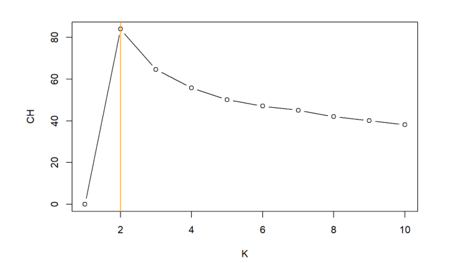
The “appropriate” K corresponds to the largest value of CH. This shows that an optimal number of clusters is K = 2.

The silhouette plot is used to assess cluster coherence. Observations with high silhouette values are much closer to their own cluster members than the members of other clusters. Observations with low (or even negative) silhouettes are close to other cluster members and thus may have ambiguous cluster membership.

Using the silhouette function in the cluster package, we find the silhouette width by inputting two arguments, clustering data and distance matrix computed using Euclidean distance.

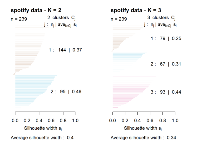
The average Silhouette for K=2 is larger than the average Silhouette for K =3. Hence, Clustering K = 2 is better.

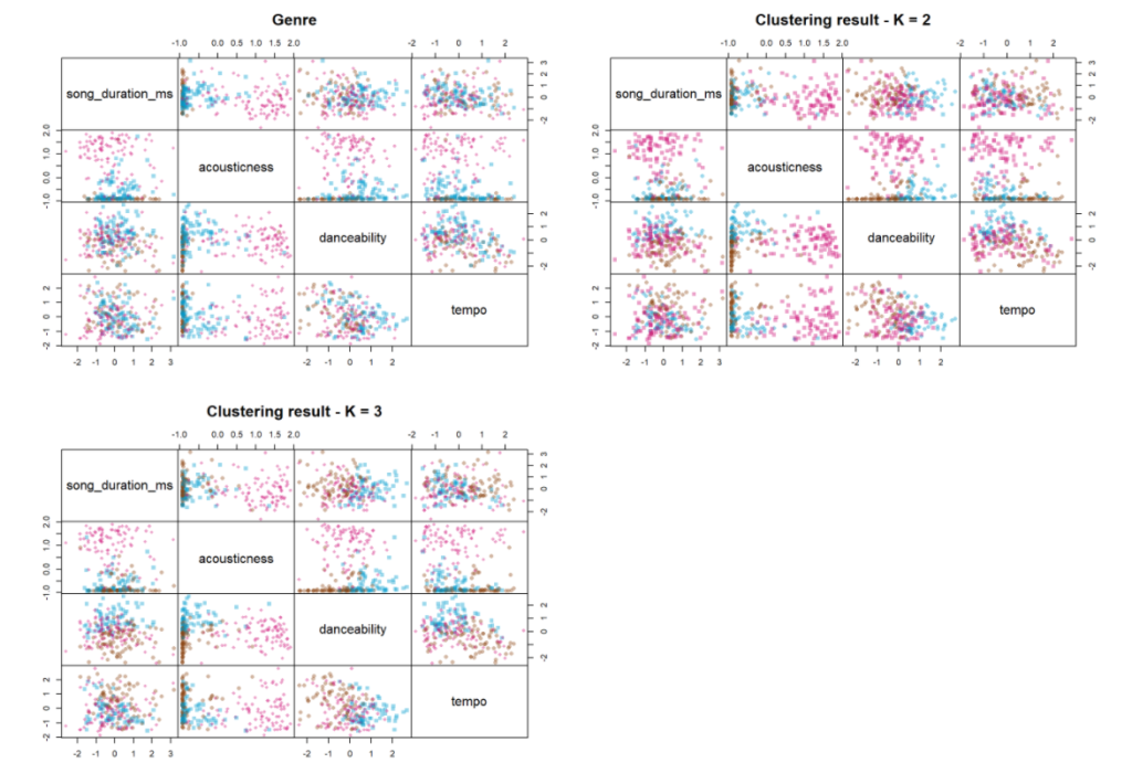
By comparing the clustering obtained to the classification into genres, we could observe that the clustering is almost similar to the genre of the given data.

We could assess the accuracy by measures of external validations like the RAND index and Adjusted RAND index. However, I have not covered that in this blog. You can have a look at that here.

The Rand index has a value between 0 and 1, with 0 indicating that the two data clusterings do not agree on any pair of points and 1 indicating that the data clustering is exactly the same. Here we have a rand index of 0.72 for K = 2 and 0.75 for K = 3. Both these values are almost near 1 hence suggesting K-means clustering using audio features of data is similar to the real clustering of data according to its genres.

The Adjusted Rand Index is used to measure the similarity of data points presented in the clusters i.e., how similar the instances that are present in the cluster. So, this measure should be high as possible else we can assume that the data points are randomly assigned in the clusters. Here ARI = 0.46 for K=2 and 0.451 for K=3, which is a relatively good measure.

Summary

To summarise, the K-means clustering algorithm:

• aims to group similar data points into clusters
• requires a choice for the number of clusters
• iterates between two steps, allocation and updating.

Further Reading

I found this blog useful for learning about the implementation of the K-means algorithm in R. To read about how to implement the K-means algorithm and other clustering methods in python you can click here. Also, to understand K-means clustering in a simpler way, this video can be helpful.