Metric Learning For Simulation Analytics

Reading Time: 5 minutes

Usual output analysis of simulations, which is done at an aggregate level, gives limited insight on how a system and its performance change throughout the simulation. To gain greater insight regarding this, you can think of a simulation as a generator of dynamic sample paths. When we consider that we are in the age of “big data”, it’s now pretty reasonable to keep the full sample path data and to explore how to use it for deeper analysis. This can be done in a way that supports real-time predictions and reveals the factors that drive the dynamic performance.

In this post, we’ll look at the emerging field of simulation analytics.

1. What is simulation analytics?
2. Metric learning for simulation
3. A simple example
4. Some final thoughts

1. What is Simulation Analytics?

The idea of simulation analytics was first described by Barry Nelson. It is not just “saving all the simulation data” and then applying modern data-analysis tools. It explores the differences between real and simulated data. Nelson outlines that the objectives of simulation analytics are to generate the following:

1. dynamic conditional statements: relationships of inputs and system state to outputs; and outputs to other (possibly time-lagged) outputs.
2. inverse conditional statements: relationships of outputs to inputs or the system state
3. dynamic distributional statements: full characterization of the observed output behaviour
4. statements on multiple time scales: both high-level aggregation and individual event times
5. comparative statements: how and why alternative system designs differ

2. Metric Learning for Simulation

The remainder of this post is a discussion of the work done by one of my STOR-i colleagues, Graham Laidler and his supervisors.

We can use sample path data available to build a predictive model for dynamic system response. In particular they use k-nearest-neighbour classification of the system state with metric learning to define the measure of distance [1] . In kNN classification, a simple rule is used to classify instances according to the labels of their k nearest neighbours.

From this definition, the paper uses

• binary labels y_i \in \{0,1\}
• instance x_i  is the system state at time t_i . More specifically, this refers to some subset of information generated by the simulation up to time t_i .

The classification for an instance x^* is

\hat{y}^* = \begin{cases} 1, & \text{if} \sum_{i=1}^k y^{*(i)} \geq c \\ 0, & \text{otherwise}, \end{cases}

where c \in [0, \infty) is some threshold and y^{*(i)} \text{ for } i = 1\cdots k are the observed classification labels that correspond to the k instances nearest to x^* . In words, if c or more of the k nearest neighbours to x^* are observed to be 1, then y^* is classified as 1 by the model.

The discussion then turned to the idea of quantifying the similarity of instances since nearest neighbour classifiers assume that instances that are similar in terms of x are also similar in terms of y . The authors attempt to fully characterise the system by including multiple predictors in their kNN model. Because of the multi-dimensionality of x_i , all variables may not be comparable with respect to scale or interpretation, so using the Euclidean distance is not appropriate.

So we now look at metric learning, which automates the process of defining a suitable distance metric.

The aim of metric learning is to adapt a distance function over the space of x . The paper uses Mahalanobis metric learning which has a distance function parametrized by M , a symmetric positive semi-definite matrix. The metric learning problem is an optimization which minimizes, with respect to M , the sum of a loss function to penalize violations of the training constraints under the distance metric and a function which regularizes the values of M . The metric learning task is subject to similarity constraints, dissimilarity constraints and relative similarity constraints which are set based on prior knowledge about the instances or using the class labels.

3. A simple example

To evaluate the model, the authors create a formulation of the problem. In this formulation, the similarity and dissimilarity constraints are partly based on LMNN[2]. Because of the high-dimensional input, a global clustering of each class may not be appropriate, so a local neighbourhood approach was used when defining these constraint sets. The local neighbourhood of an instance x_i was defined as the q nearest points in Euclidean distance. Points in that local neighbourhood are classified as similar if they had the same y value and dissimilar if they did not. The aim was to minimise the sum of squared distances of instances classified as similar while keeping the average distance of dissimilar instances greater than 1. They set the local neighbourhood size q = 20 and k = 50 nearest neighbours.

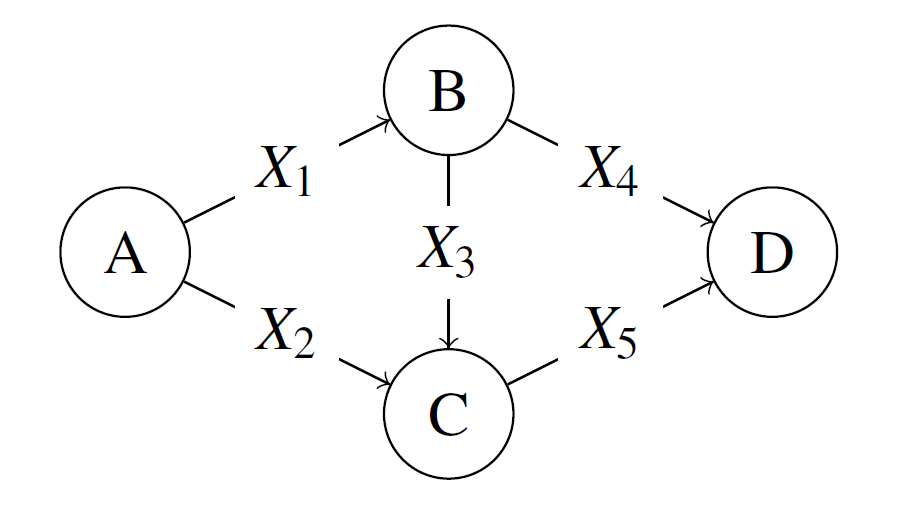
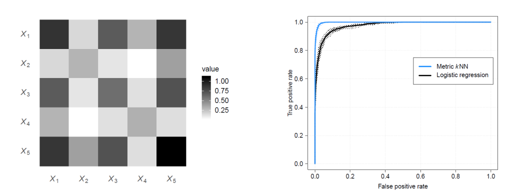
One of the illustrations they applied it to was a simple stochastic activity network. The input space was the 5 activity times and the output was whether the longest path length is greater than 5. The activity times were i.i.d X_i \sim Exp(1) . 10000 replications of the network were run. Because the data generating mechanism is exactly known, this example was useful for evaluating the model since the authors understood what the output M should reveal.  

The diagonal elements of M indicate the weight given to the difference in each variable in the classification of instances as similar or not. From the results, X_1, X_3, X_5 were the most relevant, as was expected from the intuition of the problem. The off-diagonal terms of M indicate impact of interaction terms. Using the 2-5 fold CV, metric kNN model was a better classifier than a logistic regression model.

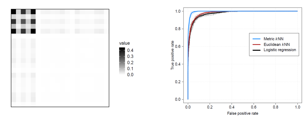
The authors then added noise variables to the model. This makes the model more realistic since multi-dimensional characterizations are likely to include variables that have little or no relationship to the output variable. Metric learning was able to filter out the noise variables while still detecting the relationship between the 5 initial variables.

4. Some Final Thoughts

I believe this solution is valuable for 2 main reasons:

1. It proposes a method for more in-depth analysis of simulation results which may be useful for real-time predictions and identifying drivers of system performance. The method is useful for revealing relationships between different components of the system and their effect on performance.
2. The method allows us to apply kNN on high-dimension input data without the needing to manually trim the state space. This allows analysis to be done without prior knowledge about what variables may or may not be relevant, as they can all be included and the metric learning will reveal the relevance.

Learn More

[1] Hastie, T., R. Tibshirani, and J. Friedman. 2009. The Elements of Statistical Learning: Data Mining, Inference, and Prediction. 2nd ed. New York: Springer.

[2] Weinberger, K. Q., and L. K. Saul. 2009. “Distance Metric Learning for Large Margin Nearest Neighbor Classification”. Journal of Machine Learning Research 10(9):207–244.