

It’s interesting that there are some problems that the younger generation, if they even know it exists, assume have been dealt with completely. That’s what I thought about lead piping. Yet the University of Edinburgh and Scottish Water have ongoing research related to this.
It became relatively common knowledge in the 1970s that lead is dangerous. However before its harmful health effects were discovered, lead was commonly used in water pipes. In Scotland, the water supplies do not naturally have high lead levels. Since the banning of lead pipes in 1969, Scottish Water has worked to remove lead pipes from the mains distribution system although some pipes carrying water to customers’ houses may still be made of lead and require replacement. Additionally, properties built before 1970 are at higher risk of containing internal lead piping or tanks and having contaminated tap water.
- What is the problem?
- What is count regression?
- Why a zero-inflated model?
- Other considerations
1. So just find and replace all the pipes…
In a world without limitations, Scottish Water would visit every household built before 1970 and test their tap water for lead-contamination. However that is not possible in reality. So instead it makes sense to model which areas (for example postcodes) have more houses with lead-contaminated water so that sampling efforts can be focused there. The goal is to identify the possible factors which increase the risk of more households in a postcode returning water samples with lead concentration greater than 1μg/L.
Data
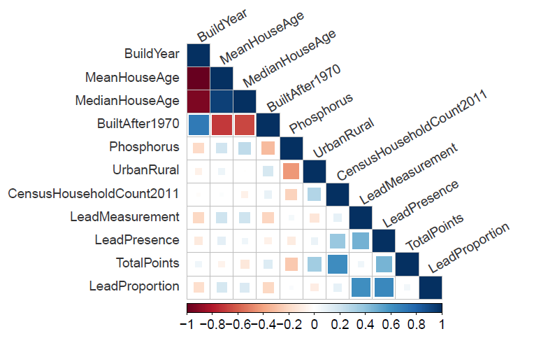
To look at this problem, we consider data containing 308 observations, each representing a different postcode. The variables included are:
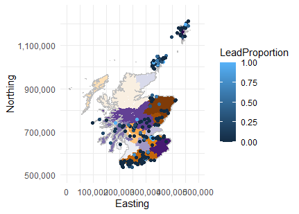
- Location related variables: water operational area, region, postcode area and district; the coordinate location of the postcodes.
- Scottish Water data: an indicator variable for if the postcode’s water is phosphate dosed and the dosage measured; an indicator variable for if old supply pipes have been replaced*.
- Census data: the 2011 census households count; the Urban Rural classification code (2-fold and 8-fold).
- Property Age related variables
- Presence of lead: number of households sampled, number of samples with lead concentration > 1μg/L (lead presence count).
2. What is count regression?
Simple regression has a response variable that can take any real value. The models we want to use need to account for the fact that the data are non-negative integers. There are some regression models specifically for count data.
Poisson Regression
Naturally when doing any model testing, we start with simplest – which is Poisson regression for count data. The response variable conditional on the regressors is Poisson distributed with mean parameter connected to the regressors and parameters by the exponential mean function.
Despite the name of the model, it is not necessary for the response variable to be Poisson distributed (marginal vs conditional distribution). However, for valid statistical inference it is necessary for the conditional mean and expectation to be equal (as is expected for the Poisson distribution).
Negative Binomial Regression
When the conditional variance exceeds the conditional mean, the data is said to be overdispersed. The negative binomial model is a standard approach to address overdispersion. It includes a dispersion parameter, \alpha which is also estimated. Similar to the Poisson model, the data does not need to follow the negative binomial distribution as long as the mean and variance are correctly specified.
3. Why a zero-inflated model?
Let’s take a step back and think about the problem for a moment. The reason many people don’t know lead piping is still an issue (aside from youthful ignorance) is that well… it’s been dealt with for the most part. So in reality many of the postcodes won’t have any households with lead contaminated samples.
This is a situation where count data may still have more zeroes than predicted by a parametric models even when using a distribution like the negative binomial. In a zero-inflated count model, the processes generating the zero counts and the positive counts are not constrained to be the same.
The zero-inflated model specifies
Pr[y=j] = \begin{cases} \pi + (1-\pi)f_1 (0), & \text{if}\ j=0 \\ (1-\pi)f_1 (j), & \text{if}\ j>0 \end{cases}The model is a mixture of a count model and a probability mass function degenerate at zero. The proportion of zeroes added (\pi) may be determined by a binary outcome model or be set to a constant.
4. Other considerations
To account for some of the variation related to location, random effect terms were added to each of the models selected. For variables like these, random effects were more appropriate than fixed categorical variables.
If you read the first section closely, you’ll remember that included in the data was an indicator variable for if old pipes have been replaced. And you’d think, well there you go! However this actually wasn’t included in the modelling at all. That’s because it wasn’t clear if the sample was taken before or after the supply pipe was replaced. So we couldn’t really infer whether any contamination recorded was already dealt with or if it was caused by internal lead pipes.
5. Conclusion
So in the end, I chose a zero-inflated negative binomial model with a random effect. This model handled both the overdispersion and the zero-inflation in the data. It is also more generalisable that the zero-inflated Poisson model. For example, if more extensive sampling is done, the data may be more or less overdispersed than the current sample and a Poisson model would not account for that.
The model identified 2 factors that have a large impact on the risk of a postcode no being free of lead contamination: whether or not a postcode receives its water from a WTW which conducts orthophosphate dosing and whether a postcode is in urban or rural Scotland. By considering these 2 major factors, further sampling can be done in postcodes that are classified as urban and are not orthophosphate dosed.
Learn more
- Scottish Water – Lead and Your Water
- Cameron, A. Colin, and Pravin K. Trivedi. 2013. Regression Analysis of Count Data. 2nd ed. Econometric Society Monographs. Cambridge University Press.
- R package – glmmTMB
Interesting stuff. I look forward to your findings and if my pipes need changing
This is very insightful and well researched!