In this post, I’d like to talk about a very unique discipline in statistics called Extreme Value Theory (EVT). Throughout my undergraduate degree, it seemed that all courses in statistics were concerned with modelling the “usual”. For the most part, this is true as statisticians in many disciplines are typically concerned with the behaviour of data on average. Why extremes is so unique is that it is looking to model the unusual. EVT looks at family of distributions which help us to gain insights into the most rare of events such as floods, earthquakes, heatwaves and more. EVT can use historical data to provide a framework which can estimate the most extreme anticipated forces that may impact upon a designed structure. Clearly, this becomes very important when designing preventative measures against such events. In this post, I’m going to give a brief introduction into EVT.
The Problem
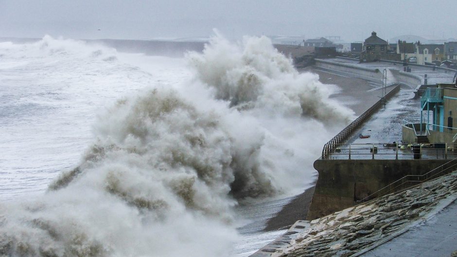
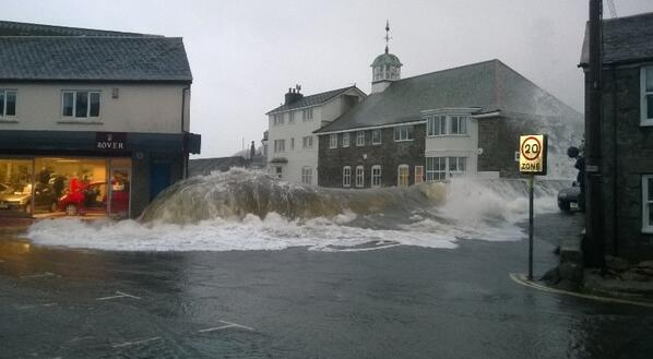
Of course, extreme events don’t happen often and so, often what’s needed is an estimate of events more extreme than what has already occurred. This involves prediction of unobserved levels based on observed levels. As an example for the need for this extrapolation, suppose a new sea-wall is required in Newlyn, Cornwall to protect against such events as pictured above which occur with extremely high sea levels. This wall may need to protect against any extreme sea levels which may occur in, say, the next 100 years. However, we may only have access to 10 years worth of historical data for the area. Thus, the problem is to estimate the sea-levels which may occur in the next 100 years based on the last 10 years of data. EVT provides families of models which allow for such extrapolation.
Classical Extremes
Continuing with the sea-levels example, suppose we have X_1, X_2, \ldots a sequence of 3-hourly sea-surge heights at Newlyn. We assume X_1,\ldots,X_n are independent and identically distributed random variables and let M_n = \max \{X_1,\ldots,X_n\} be the maximum sea-surge over n observations. These are called block-maxima and the family which is used to model these maxima is called the Generalized Extreme Value (GEV) distribution which (if you’re interested) is given by:
G(z) = \exp\left\{-\left[1+ \xi \left(\frac{z-\mu}{\sigma}\right)\right]^{-1/\xi}\right\}defined on \{z: 1+\xi(z-\mu)/\sigma > 0\}, -\infty < \mu < \infty, \sigma > 0 and -\infty < \xi < \infty.
Now, there are a few problems with this approach. Since we’re looking at blocks of n observations, say, monthly or annual maxima, there is the obvious problem that some blocks may have a larger number of extreme observations than others and there is a chance that some of these extra extreme observations could actually be larger than the maximum of another block but since they are not the maximum of the block in which they lie, they are not included in the modelling procedure. Clearly, there is a significant wastage of data here.
There are clear problems with defining extreme events as the largest observations which occur in a block. Thus, we need a more flexible way of defining extreme events.
Threshold Models
Threshold models provide this flexibility. We now denote events as extreme if they exceed some high threshold u. Exceedances of a high threshold are then said to follow another distribution known as the Generalized Pareto Distribution (GPD) which (for those interested) is defined as follows:
For large enough u, the distribution function of (X-u) conditional on X > u is approximately:
H(y) = 1 - \left(1 + \frac{\xi y}{\tilde{\sigma}}\right)^{-1/\xi}defined on \{y: y > 0 \hspace{0.3cm}\text{and}\hspace{0.3cm} (1 + \xi y/\tilde{\sigma}) > 0\}, where \tilde{\sigma} = \sigma + \xi(u-\mu).
This approach clearly provides a much more flexible approach for the definition of extreme events as well as reducing the wastage of data.
What’s next?
So far, with both of these models, we have been assuming an underlying sequence of independent observations. However, when thinking of extreme events such as high sea-levels or storms, it’s clear that these wouldn’t occur in single observations. For example, in the case of the 3-hourly sea-surge measurements at Newlyn, if an extreme event occurred, i.e the sea level was very large , we would not expect the sea-level to return to normal after a single observation. It’s more likely to be high over a number of observations. Thus, the assumption of independence between observations is unlikely to be valid. In fact, for most type of data where EVT is applied, independence in time is unrealistic.
In the next post, I will discuss the use of stationary sequences to approximate this short-term dependence between observations in time series extremes.
I hope you enjoyed this brief introduction to the two main approaches to modelling in EVT. Thanks for reading!