
In this blog post, I’d like to talk about the importance of experimental design in simulation studies. Simulation studies are widely used in modern scientific research as they attempt to model real-life situations. Models can be very complex and can include a huge range of factors and sources of uncertainty. Design of Experiments (DOE) may seem like an obvious step when constructing a simulation experiment but the extra effort involved in constructing an efficient design can be off-putting and thus, sometimes, the benefits of DOE are not utilised. DOE, in essence, is about building your simulation experiment in the most suitable way possible for the situation.
Motivation
To demonstrate the importance of DOE, we will look at the developments in supercomputer capability in the last decade or so. In June 2008, a supercomputer called the “Roadrunner” was unveiled. With a cost of $133 million, this machine was capable of doing a petaflop (a quadrillion operations per second). Five years later, China took the position as the world leader with the “Tianhe 2” supercomputer which had a capability of over 33 petaflops. Today, the “Fugaku” supercomputer built in Japan holds the title with a capability of over 440 petaflops. Even with these massive capabilities, efficient DOE is still extremely important. Suppose we want to run a simulation with 100 factors, each with two levels (low and high) of interest. Looking at all possible combinations of the 100 factors and assuming that each of the 2^{100} runs consisted of a single machine operation, a single replication would take over 40 million years on the “Roadrunner”, over 1.1 million years on the “Tianhe 2” and even with the massive capability of the current world-leader, a single replication would still take over 90 millenia.
Clearly, no-one has 90000 years to wait for the results from a simulation experiment! With some simple screening designs, the computation time can move from millenia on a supercomputer to days or even hours on an “everyday” computer.
Example
Factorial designs are a simple starting point when looking at DOE. They explore all possible combinations of the factor levels. The simplest design (mentioned above) is the 2^k factorial design which requires only two levels for each factor. In DOE, the idea is to construct a design matrix which represents all of the combinations of factors being assessed in the experiment. In the design matrix, every column corresponds to a factor and the entries within a column correspond to levels of the factor. Each row of the matrix represents a combination of factor levels called a design point.
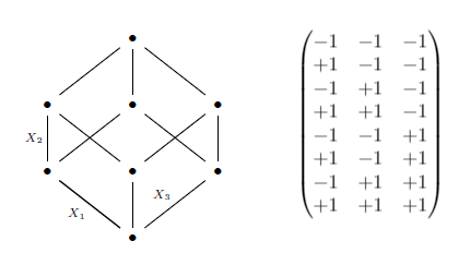
For example, let’s look at the 2^3 case, where we are assessing 3 factors, each with 2 levels “low” (denoted by -1) and “high” (denoted by +1). The first column of the design matrix alternates between -1 and +1 , the second column alternates -1 and +1 in groups of 2 and the third in groups of 4 (with higher numbers of factors, this would continue in the same manner by powers of 2). This equates to sampling at the corners of a hypercube, as below. The columns in the matrix correspond to X_1, X_2 and X_3 respectively. The factorial design can also look at interactions between these factors. An interaction is added to the design matrix by simply multiplying the corresponding columns of individual factors in the interaction.
As demonstrated above, this design can be computationally expensive when the number of factors is large. Finer grids which incorporate more levels for each factor also have the same problem.
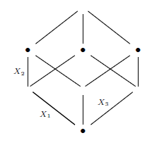
One variation of this design that can be useful is a fractional factorial design. This approach samples at chosen fractions of the corner points of a hypercube. Below is a graphical depiction of a 2^{3-1} fractional factorial design. In this case, three factors are examined again, each at two levels but the number of design points (rows in the matrix) is only 4 instead of 8. Two points lie on each of the left and right faces of the cube with each face having one instance of X_2 and X_3 at each level allowing us to isolate the effect of X_1. Averaging results for the top and bottom faces isolates the effect of X_2 and the front and back faces allow us to look at X_3.
The gains in efficiency are massive! Going back to the supercomputer example, running the 2^{100} full factorial design would take over 40 million years on the “Roadrunner”. However, running a 2^{100-85} fractional factorial design with only 32768 design points on the same machine would take less than a second!
Conclusion
This has only scratched the surface of experimental design but some of the benefits of efficient DOE are evident. There are many more examples of potential designs and much more insight to be gained when an experiment is designed in the most suitable way for the data and research questions we want to answer. If you’re interested in reading more about DOE, the paper below details many more examples of designs and their strengths/weaknesses. Thanks for reading!
WORK SMARTER, NOT HARDER: A TUTORIAL ON DESIGNING AND CONDUCTING SIMULATION EXPERIMENTS – S. M. Sanchez & H. Wan