You’ve probably heard a lot about “particle filtering” in the last few years in the context of mask wearing. What you might not know is that particle filtering is also the name of a family of algorithms useful in epidemiology – in this context, “filtering” refers to statistical inference on quantities that cannot be observed directly and the “particles” are simulated possibilities for this hidden information. Particle filtering is used for inference on noisy or partially observed data – for example, in the epidemiology context the spread of a disease can be modelled as a random process which we can only partially observe, since not all infected individuals can be tested for the disease and tests are not 100% accurate.
Estimating true case numbers and monitoring the transmission rate of a disease are vital to understanding and containing its spread – in the COVID-19 pandemic such statistical analyses have been critical in informing government policy. As such, there has been much interest recently in using particle methods to analyse COVID-19 data. This blog post will introduce the filtering problem in the context of analysing a small simulated epidemic dataset, focusing on the task of predicting the true number of cases at a given time.
Epidemic Modelling
Our running example will be a realisation from the Reed-Frost epidemic model: we introduce a disease to a closed population of fixed size N and monitor who is susceptible (S), infected (I), or recovered (R) as time goes on. Initially, all are susceptible to the disease, meaning they can become infected by contact with an infectious (I) individual. After they recover from the disease they are classified as removed (R) and cannot be infected again. It is assumed that the infectious period of the disease is short compared to its incubation period, so that individuals infected at time t will infect others at time t+1 and then recover. We assume for simplicity that all susceptible individuals independently have probability p of coming into contact with and being infected by any given infectious individual in this time. The epidemic will begin with the introduction of a single infectious individual at time 0.
Putting these assumptions together, the number of infections at each timestep will be binomially distributed, with parameters depending on the current number of susceptible individuals and the probability each one has of being infected. If we denote the number of susceptible individuals at time t by S_t and the number of new infections by I_t, we can consider the unobserved “hidden state” in the process to be x_t = (S_t, I_t), since the number of recovered individuals at time t can be computed from I_t and S_t as R_t = N - S_t - R_t.
The probability of any one susceptible individual escaping infection at time t + 1 is (1 − p)^{I_t}, since they would have to avoid contact with each of the I_t infectious individuals to escape infection. The distribution of new infections at each timestep t \geq 1 is I_{t+1} | (S_t, I_t) ∼ \text{Binom}(S_t, 1−(1−p)^{I_t} ), with S_{t+1} = S_t −I_{t+1} since the recently infected people are no longer susceptible to the disease. Since the epidemic starts with the arrival of a single infectious person, we have that I_0 = 1 and S_0 = N.
This model describes the underlying dynamics of the disease, but in a real epidemic we have an additional complication – at no point can we directly observe I_t or S_t! We will assume a fixed probability p_{obs} of detecting any given infection, reflecting how likely an infectious individual is to take a test and how likely the test is to detect the presence of the disease. This means that the number of cases we actually observe (we’ll call this y_t) is binomially distributed, given by y_t | x_t ∼ \text{Binom}(I_t, p_{obs}).
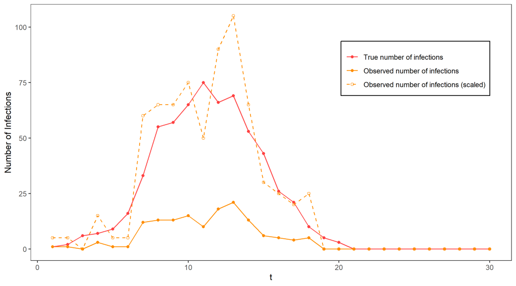
Clear as mud? To illustrate all of that, the figure above shows a simulation from this model terminating at time T = 30, with N = 1000, p = 0.0015, and p_{obs} = 0.2, which will be used as a running example. Clearly, the observed number of cases gives an incomplete picture of the epidemic, as the true number of cases reaches much higher. If we know p_{obs} = 0.2 (for the moment we will assume we do), it is tempting to estimate the true number of cases by scaling the observed case numbers by a factor of 1/0.2 – indeed, if we only had one datapoint this would be the best guess we could possibly make for the true number of cases since on average we detect 20% of infections. The dashed line on the graph indicates the outcome of using this approach – it is not too terrible as an estimate of the true number of cases but is extremely variable.
Such sudden and extreme swings in the number of cases are very unlikely in the Reed-Frost model! Ideally, we’d like to take this knowledge into account in our guesses for the number of cases. This would require using all of our observations so far to get a better idea of what the situation is like – for example, keeping track of the total number of infections detected so far would help give an indicator of how fast the disease is currently spreading – for example, at around time t=11 we can guess that over 30% of the population has already been exposed to the disease (by multiplying the total number of infections detected by 1/0.2), and use our knowledge of the Reed-Frost model to guess that this means we are close to the peak and the disease will soon start dying out.
Formally, we can use all of the available information to make inferences about the true hidden state by using the filtering distribution, a probability distribution that captures our knowledge (and uncertainty) about the hidden states at time t given our sequence of observations up to that time. We can use this distribution to compute a best guess for the true number of cases or to estimate the probability that this took a certain value. It is important to consider this as a probability distribution, since when there is randomness in the observation process it is not possible to be completely certain of what the hidden states actually were.
The Filtering Distribution
The filtering distribution is the name given to the distribution p(x_t \, | \, y_1,…,y_t), where as before x_t is the hidden state and y_t our noisy or partial sequence of observations. This can be calculated recursively – supposing we know the filtering distribution for time t − 1, we can obtain the filtering distribution for time t using Bayes’ theorem:
p(x_t \, | \, y_{1:t} ) = \frac{ p(y_t \,|\, x_t) \, p(x_t \,|\, y_{1:t-1}) }{ p(y_t \,|\, y_{1:t-1}) } \, ,
where the predictive distribution p(x_t \,|\, y_{1:t-1}) can be found by integrating (or summing if the state space is discrete, as it is in our example) over possibilities for x_{t-1} and the normalising constant p(y_t \,|\, y_{1:t-1}) by integrating over possibilities for x_t. Unfortunately, in most cases the story does not end here, as we typically cannot evaluate the required integrals exactly. Note that since the population in our running example is closed and has fixed size, the state space for this model is finite with up to N possibilities for both S_t and I_t. This means that we can compute the exact filtering distribution by exhaustively summing over every possibility, although this can become prohibitively computationally expensive for large populations – in our small example this took six hours to calculate! This exact filtering distribution is represented below, and we can see right away that its mean is a much better guess for the true number of cases than we got by just scaling up the observed number of cases.

We will explore what to do when the exact calculation is not possible (or is computationally infeasible) in part 2 of this post, and we will see that in our example a very good approximation can be obtained in mere seconds.
Further Reading
- How NASA used the Kalman Filter in the Apollo program – Jack Trainer
- An Introduction to Sequential Monte Carlo Methods (chapter 1) – Arnaud Doucet, Nando de Freitas & Neil Gordon