This is the second part of a series on using particle filtering in epidemiology. In part 1 we saw an example of how to model observed case numbers as a partially observed random process and formulated the problem of inferring the true case numbers as a filtering problem. Unfortunately, exact inference is rarely possible for realistic models and was very computationally expensive even in our relatively simple example! This post will introduce the bootstrap particle filter, an approximate method that is much more computationally efficient and can be used in cases where it is not possible to compute the true filtering distribution.
Sequential Importance Sampling
A common way of dealing with intractable integrals or complicated probability distributions is by using Monte Carlo methods – in our case, we can simulate from the probability distribution p(x_t \,|\, y_{1:t-1}) for x_t since we know the dynamics of the disease (we can do this sequentially by simulating x_t from time 0 up to t according to the binomial updates we defined earlier). We can also compute p(y_t \,|\, x_t) directly since we know the distribution of the observation process. These are the ingredients required to use the Monte Carlo technique of importance sampling to approximate the filtering distribution – if we simulate a large number of samples (known as “particles”) for x_t we can weight them proportionally to p(y_t \,|\, x_t) and estimate properties of the distribution (for example, the mean) by treating our weighted particles as if they were a sample from the filtering distribution.
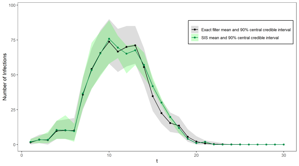
Unfortunately, it is quite inefficient to use importance sampling out of the box in this setting – most of our simulations will not be close to what really happened in the epidemic and will therefore have very small weights. We need to find a lot of plausible possibilities for the true sequence of case numbers in order to get a good estimate for the filtering distribution, otherwise we will just end up being very overconfident about the one particle we simulated that is somewhat close to the truth. This problem gets worse at each timestep as the number of possibilities for the path taken by the hidden states increases – In fact, the number of particles required to produce good estimates increases exponentially in t. In our epidemiology example (see below for a comparison of the estimated filtering distribution with the true distribution) importance sampling did well initially but the shrinking credible intervals after t = 10 indicate that the sample weights are becoming increasingly concentrated on just a few particles.
One issue with this approach is that we keep and use all of the particles, no matter how unlikely they are to be close to the truth. For example, in our epidemic we know that the true number of cases must be at least as big as the number of cases we observed, so any simulated particle that does not satisfy this at each time point will have a weight of 0 since it cannot possibly reflect the true number of cases.
The Bootstrap Filter
The bootstrap filter is a way of sequentially generating particles that are more concentrated in areas of high density of p(y_t \, | \, x_t). Instead of continuing to propagate all of our particles forward and sequentially updating their weights, the bootstrap filter uses the weights to resample the particles, creating a new generation of particles that can all be given equal weight. This allows particles with negligible weight to be eliminated, while we simulate several descendants of the particles with higher weights. At each timestep, we sample the next generation of particles independently and with replacement, with each particle having a probability proportional to its weight of being selected.
We’ll illustrate this on our running example via an animation – the gif below shows the propagation of 4 particles, with the true number of cases indicated by the dashed line. The dots representing each current particle are scaled according to their weights, with x’s indicating removed particles. The resulting estimate of the filtering distribution is shown at the end.
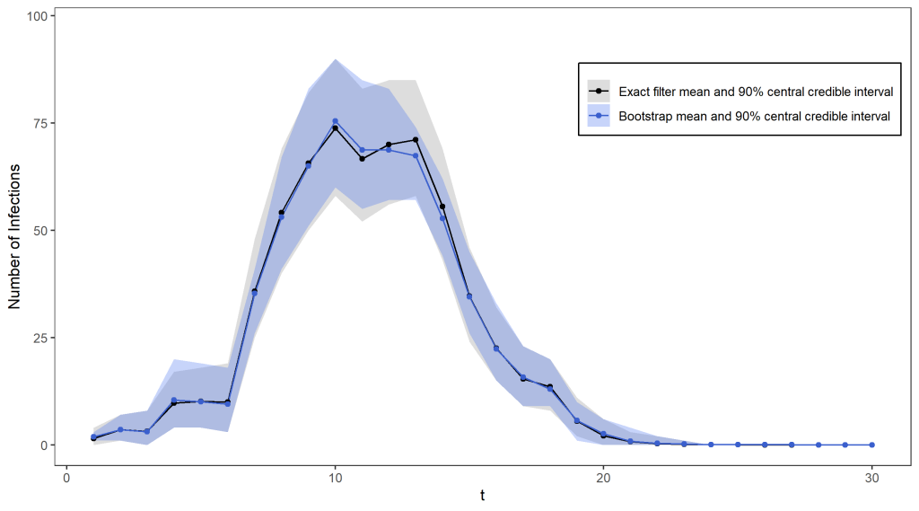
Using 100 particles (see the figure below), we obtain a pretty reasonable approximation for the exact filter mean and quantiles, and for over 1000 particles the two are virtually indistinguishable. The only difference is that the bootstrap filter algorithm takes only seconds to run (even with a huge number of particles), while the exact distribution took several hours to compute!
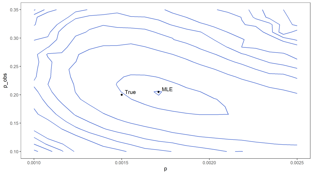
In addition, the weights within the particle filtering algorithm can be used to estimate the data likelihood. If we do not know the true values of p and p_{obs} this can be used to estimate which values are likely given our data as we can run the particle filter for different possibilities for the parameters. For example, we can roughly locate the maximum likelihood estimators in our example by estimating the data likelihood on a grid of possible parameter values (see below for an approximate contour plot of the likelihood, with the rough location of the maximum indicated).
Optimising for estimates of p and p_{obs} is easy enough to do in our simple example with only two parameters, though much harder for more complicated models. Also, just estimating the parameters isn’t enough if we also want to perform inference on the hidden states, since simply substituting these into a particle filter wouldn’t reflect the fact that we are uncertain about what the true parameter values are – our uncertainty about the parameters results in a higher degree of uncertainty about the hidden states. A neat way of performing inference on the parameters and hidden states jointly is by using particle Markov chain Monte Carlo.
Further Reading
- How could particle filter track Thanos? – explaining particle filter without mathematics – Ziyang Yang
- A Tutorial on Particle Filtering and Smoothing: Fifteen years later – Arnaud Doucet and Adam M. Johansen