
In the previous blog post we looked at the infamous Monty Hall problem and its controversial (but correct) solution. The main problem has been talk of countless blog posts, news articles, and youtube videos; providing a nice introduction to probability and Bayes theorem. And while it is fun to rehash the same story, it might be worth looking at how to broaden the problem and see how the same core principles can be applied to a more obtuse setting. With this we can explore some of these re-formulations, starting with expanding the number of doors in our game.
Monty Hall: Live from the Hilbert Hotel!
Let’s envision the following fictitious scenario; in which after the success of his three door final showdown, Monty and his team have been gifted a bigger budget to make a more elaborate show, and a new, possibly infinitely big studio. Here, Monty utilises this increased budget to order his producers to purchase more doors. Now that he possesses a studio filled to the brim of disused doors, Monty again places one car behind a door and keeps count of where it is placed. While a flood of goats trundle in and hide behind the rest, he asks a contestant, now slightly more intimidated than their predecessors (see below gif), to pick a door. The contestant hesitantly chooses, giving way to our host opening every door but the contestants and one final door.

Now we again pose the question, stick or switch? Given the information we attained from the original Monty Hall situation, it makes sense to have an intuitive guess that switching will be in the contestants best interest. And we can test this again by using Bayes’ Theorem and some basic Probability theory.
Like in the original incarnation, we define events and variables for the new version. Instead of 3 doors, we now possess d doors. Each of these doors are assigned the event it may possess the prize behind it, we can define these events as D_1,...,D_d. While also allowing G to be the event we open all but doors 1 and d to reveal a goat. So with this in mind, we can formulate the following Bayes equation for any door in particular, say i:
\mathbb{P}[D_i|G]=\frac{\mathbb{P}[D_i]\mathbb{P}[G|D_i]}{\mathbb{P}[G]}.The individual probabilities for the right hand side are calculated as:
\mathbb{P}[D_1]=...=\mathbb{P}[D_d]=1/d \\ \mathbb{P}[G|D_1]=\frac{1}{d-1} \\ \textrm{(As we are just restricted to opening every other door if the prize is here)} \\ \mathbb{P}[G|D_d]=1 \\ \textrm{(As we are just restricted to opening every other door if the prize is here)} \\ \mathbb{P}[G|D_2]=...=\mathbb{P}[G|D_{d-1}]=0 \\ \textrm{(If the prize lies in all these doors we want to open, we clearly can’t open them).}Since D_1 to D_d cannot occur simultaneously, then we can use some more simple statistical properties, specifically mutually exclusivity, to express the probability of a goat behind all but doors 1 and d as follows in this slightly long, but hopefully intuitive derivation:
\mathbb{P}[G]=\sum_{i=1}^d \mathbb{P}[D_i]\mathbb{P}[G|D_i]\\= \mathbb{P}[D_1]\mathbb{P}[G|D_1]+ \mathbb{P}[D_d]\mathbb{P}[G|D_d]+\sum_{i=2}^{d-1}\mathbb{P}[D_i]\mathbb{P}[G|D_i]\\ =\frac{1}{d}\cdot \frac{1}{d-1}+\frac{1}{d}\cdot 1=\frac{1}{d}\left(\frac{1}{d-1}+1\right)=\frac{1}{d}\left(\frac{d}{d-1}\right).Remember we opened all but door 1 and d, so all doors in-between will have a probability 0 of having the car behind it. Thus, we substitute the above derivations back into Bayes Theorem equations, but only for doors 1 and d are,
\mathbb{P}[D_1|G]=\frac{1/d\cdot (1/d-1)}{1/d\cdot d/(d-1)}=\frac{1}{d} \\ \mathbb{P}[D_d|G]=\frac{1/d\cdot 1}{1/d\cdot d/(d-1)}=\frac{d-1}{d}While tedious, this derivation is pivotal in allowing a generalisation of the problem. Generalisations are crucial in mathematics, allowing us to expand our problem from an initial set of constrained numbers (like only 3 available doors) to as many doors as we want, and all we need to do is plug that number into d.
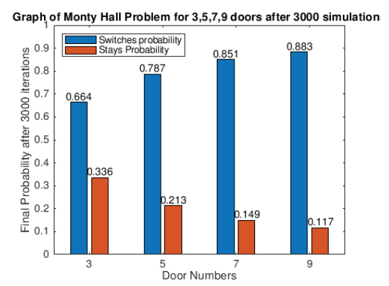
To test this – and provide a little sanity check – we can hark back to our original Monty Hall Problem and seeing that substituting 3 doors gives us probabilities of switching and staying as 2/3 and 1/3 respectively. So now we have a rather straightforward method to show, no matter how many doors we have, if we open all but one door and the original door, it is in our best interest to switch. In addition to this, although trivial to point out, we see that with more doors, our likelihood of winning when switching increases. For example, with d=7 doors, we should, by plugging our values in, attain the staying probability (i.e. door 1) as 1/7, and switching (to door d) as 6/7.
To see this in practice let’s run some simulations for 3, 5, 7 and 9 doors after carrying out Monty Hall’s deal 3000 times.

Winning isn’t everything
Our second generalisation into Monty Hall’s problem is one in which we are looking to try flip the odds back into the favour of the host. Given the generosity of winning when we expand the problem to d doors, it is now worth seeing if limiting the number of doors Monty opens can make it more – or less – likely for the contestant to win when switching. If we think about this in a logical manner, it should be the case that now we have the option of which door we can switch to, we are less likely to get the prize than in the previous scenario if we switch. But it is worth calculating how much of a detriment this new rule is to our contestant. And analysing how drastically our odds can change by opening less and less doors.
This time we will take a scheduled commercial break out of laziness to relieve ourselves of any more probability equations and focus solely on numerical computations. Consider an example where, given d doors, we open k of these. More specifically let’s look at the case of having 10 doors and we open a subset of these, analysing the number of times we win if we switch, we win if we stay, and the new third case that we don’t win if we stayed or switched. This is seen in the following graph.
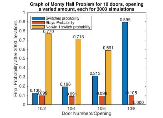
As we can see in the choice between 10 doors, when opening 8 (which is the max number of doors we can open) and opening 6 (in which we have a choice as to what we can switch to), there exists a significant dip in the probability of winning when switching, with it then being more likely to not win the game whatever we do. This is due to the truly random choice we now have with the selection of the door we might want to switch to. Despite all these changes, the chance of switching consistently gives better odds than staying. We can see this in the generalisation of opening k from a set of d doors. This is given as the following equation:
\mathbb{P}[\textrm{Winning when switching}]=\left(\frac{d-1}{d}\right)\cdot\left(\frac{1}{d-k-1}\right)For those in dire need of a Bayesian derivation (as I normally am), one can refer here. As a little test, we can take d=10 and k=2 and see that the probability of winning when switching as \approx 0.129, which leaves our simulation pretty damn close to what we want.
And with this we can conclude our investigation into suspected goat farmer Monty Hall and his mystery doors. But was this investigation as concrete as the numbers suggest?
Statistical stage fright
In these two blogs we’ve seen how applying some mathematical rigour allows us to understand, dissect and create advantages in a game of seemingly random luck. With this being said, as often is the case of applying Mathematics to the real world, our logical reasoning may still not be perfect, nor reveal the true solution to the problem. since arguments could be made in that randomising the choices of contestants in the simulation and using conditional probability detracts from the human element in the game. That in which the host, the atmosphere and the audience play a crucial role in the dilemma posed to the contestant, perhaps leading to a bias in the options available. This is something that probability and random simulations simply cannot account for. Hence it could even be contested that in reality, based on the host’s hints and approach towards the contestant, the probability of finding the winning car can range from 1/2 to 1. A paper on this dilemma of the human element can be see here.