Stochastic Simulation of Diseases: Introduction and models

“I simply wish that, in a matter which so closely concerns the well-being of the human race, no decision shall be made without all the knowledge which a little analysis and calculation can provide”

Daniel Bernoulli, 1760

A brief history of Infectious Disease Modelling

In 1766, Swiss Mathematician Daniel Bernoulli published an article in the French literary magazine Mercure de France concerning the effect smallpox had on life expectancy and the improvements which could be made with the introduction of inoculation. Bernoulli’s concluding argument, from which the aforementioned quote is derived, led to the creation of some of the first epidemiological models.

This does not mean that the paper by Bernoulli was immediately lauded by his peers. Jean le Rond d’Alembert was a prominent mathematician and intellectual at the time; albeit slightly behind the curve in probability theory, publishing in “Croix ou Pile” his rationale behind believing the chance of attaining a head in a two toss game was 2/3. D’Alembert clashed with Bernoulli on the issue, authoring a rebuttal in a 1760 paper “On the application of probability theory to the inoculation of smallpox”.

Bernoulli had initially communicated his work in a 1760 presentation in Paris. However, issues caused the paper to not be released until 1766, giving d’Alembert a head start in his critique. He argued against some of the assumptions Bernoulli had made with respect to the probability of infections and the independence between age and dying of smallpox. D’Alembert’s alternative formulation also resembles modern modelling and, despite the differing opinions, both agreed that inoculation of the population was the way forward.

Bernoulli’s submission is often regarded as the foundation to what would eventually become mathematical epidemiology, although the field as it is known today did not further develop until the early 20th century. This arrived in the form of work by the polymath Sir Ronald Ross, who wrote on malaria prevention by crafting a model of two differential equations. More generalised models were also produced by William Kermack and Anderson McKendrick , their SIR model provided early forms of compartmental modelling; a class of models that form the cornerstone of much subsequent research. These models took a deterministic form where no randomness is involved in the system and the output will always be replicated if given the same set of initial parameters.

What we are more interested in are another class of compartmental models that arrived not too long after deterministic models: stochastic models. These types of models included the effects of randomness commonly found in real-life scenarios. There has been many approaches to these, each applicable to certain areas. We consider a few of these models in this blog post, all of which revolve around compartmentalising the population into key components: Susceptible, Infected, and Recovered individuals. The idea being you leave one state and filter into the next. Thus, under these basic assumptions, recovery can also mean recovering 6 feet under in a casket. But let’s be positive and imagine all contractors of the hypothetical disease we discuss recover to live long and fruitful lives.

Chain Binomial Models

We can try garner understanding of stochastic models through the introduction of a simple, probability based method in chain binomials.

These models are discrete time (updates happen in an incremental step) and see where each fraction of the population is at the next time step. Some general yet subsequently quite restrictive assumptions are placed on the model. Namely:

1. The population is fixed.
2. Disease will always transfer whenever contact is made.
3. Contacts are independent (two people cannot infect one individual).
4. Infected people recover one time step after infection.

Obviously in reality this is not likely to hold on large scale populations, however in small, enclosed environments such as Hospitals, Schools and Households, the use for this model becomes more relevant.

So how does one model the movements between compartments? Say we infect I_t people at time t, then at the next time point we infect I_{t+1} people. These newly infected individuals will now leave the susceptible state by our assumption (2), and then by assumption (4), we must put the infectious people from the previous time step t into the recovered population. Mathematically we express this as:

S_{t+1}=S_t-I_{t+1} R_{t+1}=R_t+I_{t}

Now the most pertinent question is how do we govern the number of infections? You can perform some pretty elementary maths to arrive at the binomial distribution (for the curious page 18/19 of my Master’s thesis covers this). From a pool of S_t susceptible individuals, we find the probability of infecting x people given the probability of not infecting anyone is q. You can see why we phrase this last part in such a counterintuitive way shortly.

Deterministic, or fixed updates, can be done by taking the expectation to find infections. Conversely, if you want to incorporate an air of chaos and randomness (and you actually read the title of this post), updates can also be done stochastically through a set of Bernoulli trials.

The last step of the model is how to determine the average number of infections one infectious person is expected to give in this set up, or more commonly referred to as the basic reproduction number (\mathcal{R}_{0}). Say we have a total population of N, then,

\mathcal{R}_0=(N-1)(1-q).

The value q, which is used as a parameter in the binomial distribution to inform on the number of infections, can essentially be recovered from this reproduction number. To see chain binomial in action we can simulate an epidemic of N=500 people and a \mathcal{R}_0=1.5.

Given the stochastic nature, it may be best to run multiple simulations as to not end up with potential anomalous results informing us incorrectly on what is likely to happen. Here, 7 iterations are chosen.

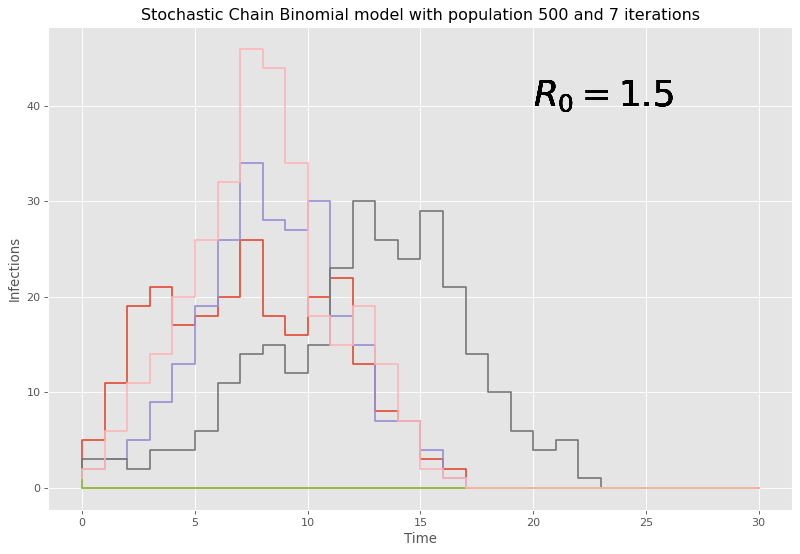
Here, given our large initial number of people, it can be seen that the chain binomial model dies out quickly with large populations and the discrete time steps lead to chunky graphs where conclusions are hard to be drawn. Therefore, this model is fairly weak and outdated to the task at hand, and it should come at no surprise that there are models that do perform better with larger populations, and a reaction based approach is considered next.

Gillespie’s Algorithm

Despite being initially formulated by the much cooler named Joseph Doob, the method was presented to the public forum by Dan Gillespie in 1976 an showcased a stochastic method to simulate the time evolution of a chemical system, through chemical reactions. This method can be stolen borrowed and applied to the epidemic setting through a re-evaluation of what these reactions can represent.

We can think of the compartments we have defined earlier and how the movement between them can be thought of as reactions between states. More specifically, two ‘reactions’ take place, an infection and a recovery. The former being a combination of a susceptible and infectious individual, and the latter being an infection contacting a recovery; which in this sense can be thought of as perhaps a healing ailment. For the algorithm itself, this poster offers a neat overview of what’s at play and includes an epidemiological example.

An interesting feature of this algorithm is its use of Monte Carlo methods to dictate what reaction takes place, and its update states in a fraction of a time. This leads to both the stochastic nature we are looking for in these methods, as well as a more advantageous update strategy when compared to the often large discrete time updates with the previous chain binomial model.

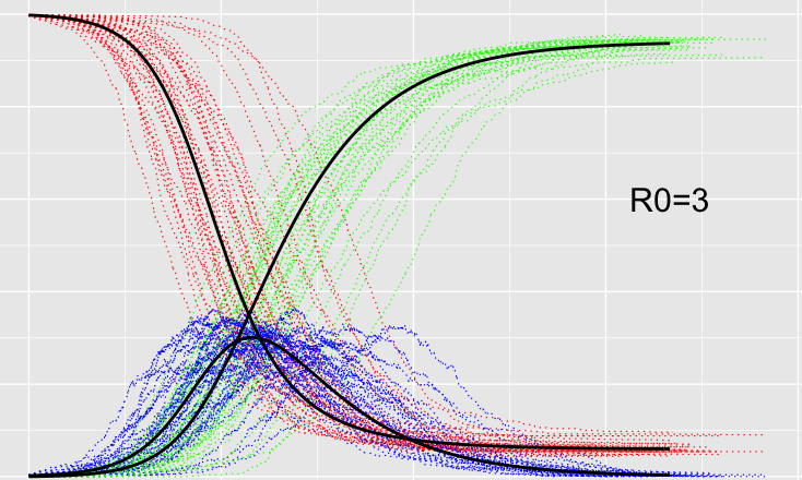
It should be noted that with fixed fractional time updates, this method can be computationally expensive to implement, so a way to calculate more efficient time steps using tau-leaping is preferred. An example using the same set up of 500 infectious individuals, but with a slightly higher reproduction number of \mathcal{R}_0=3, to compare to the chain binomial is seen below:

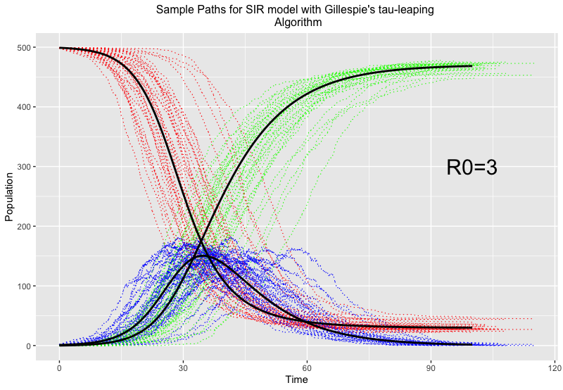
Here, red, blue and green represent susceptible, infected and recovered individuals respectively, and the thick black lines give the trajectory of the epidemic if no randomness was involved.

You can see the different trajectories (included for the same reason as the chain binomial to accompany for the effects of randomness and give us a fuller picture) vary greatly around the time of most infections, but all balance out towards the end. This method of evaluation is fairly good at epidemics on large scales, and the randomness feeds into why we’d want to use stochastic models in the first place…

Takeaways and further investigations

The use of stochastic models might not be immediately obvious, from a naive point of view why would we want models that have the potential to deviate from what we expect to happen with fixed, deterministic models? In an idealised scenario where we play god, and have a clear view of how something will progress, then models that don’t factor in randomness is a clear and obvious avenue. However, this is never the case and has been seen extensively within the last few years that there is no way to truly model and predict the behaviour of humans and the rationale behind their decisions. So modelling contacts between groups and adding unpredictability in how it might happen show, even on a small simplified scale, the range of possibilities that could still potentially happen. Where deterministic models give an idea on what should happen given a set of assumptions, stochastic models provides what could if these fail or are effected by chance.

This blog just scratches the surface of possible avenues in stochastic modelling of epidemics. Another big idea in this field is Stochastic Differential Equations based approaches, which uses ideas from Stochastic calculus and financial mathematics, a potential future blog post in the making. More on this, simulation of methods, sensitivity analysis and a use case relating to malaria, can be found in my MSc dissertation here.

References

Linda J. S Allen is a rockstar of stochastic mathematical epidemiology, even been awarded prizes for her work in the field. She has produced the following concise tutorials, as well as length books on areas of stochastic epidemic modelling:

• An Introduction to Stochastic Processes with Applications to Biology, CRC Press: www.routledge.com/An-Introduction-to-Stochastic-Processes-with-Applications-to-Biology/Allen/p/book/9781439818824
• An Introduction to Stochastic Epidemic Models, Springer Berlin Heidelberg, Berlin, Heidelberg, pp. 81–130.
• “A primer on stochastic epidemic models: Formulation, numerical simulation, and analysis”, Infect Dis Model 2(2), 128–142.

For more on the history of epidemic models, and directions to the plethora of literature on the matter, the review article : “How mathematical epidemiology became a field of biology: a commentary on anderson and may (1981) ’the population dynamics of microparasites and their invertebrate hosts” is an excellent read and is open access from here: https://royalsocietypublishing.org/doi/10.1098/rstb.2014.0307.