
Clio Johnson
The central dilemma of quantum mechanics is often how best to solve the Schrödinger wave equation in order to find the wavefunction and allowed energies of a system. This becomes much harder the larger or more complicated a system of particles gets, requiring numerical methods to solve. One such class of methods are quantum Monte Carlo (QMC) simulations, defined by their use of random number generation. At the start of a QMC simulation an initial guess must be made or generated. The convergence of QMC simulations is sensitive to the accuracy of these initial configurations. This project aimed to explore various algorithms to generate initial electron distributions within a QMC program called CASINO. The default algorithm simply placed electrons randomly within 2 Bohr radii of a given nucleus. Algorithms explored by this project included samplers with probability density functions based on hydrogenic orbitals, approximate charge densities and Slater-type orbitals.

Clio Johnson
Welcome!
My research is concerned with Quantum Monte Carlo (QMC) methods. These are methods used to solve the Schrödinger wave equation to find the total energy of and predict properties of many-body quantum systems. QMC methods have been used extensively in quantum chemistry, condensed matter physics and materials sciences. They can, in principle, be used to study any system able to be described by the many-body Schrödinger equation, but my project focused on studying systems of electrons around ions.
Throughout my project, I have sought to improve existing methods for the generation of initial distributions, electron configurations used to seed the algorithm, in order to speed up the QMC simulations. Some of my data are presented here to outline key results of the project. A brief explanation of the kind of systems being studied and QMC methods can be also found on this page.
What are QMC methods, anyway?
Monte Carlo methods are a class of numerical methods defined by their use of random numbers to approximate an value over a number of steps. In principle they are exact if left running for an infinite amount of time, but can generally reach suitable degrees of accuracy in reasonable finite times. Nonetheless, in many cases they are known to be slower than other iterative methods.
Quantum Monte Carlo methods are MC methods applied specifically to the solution of the Schrödinger wave equation, the equation which governs the behaviour of quantum systems. There are multiple different types of QMC method, each with their own advantages and disadvantages.
My project exclusively used the Variational QMC (VMC) method, which calculates a close upper bound to the ground state energy of a system.
VMC works by taking a distribution of electrons, and proposing a small change in said distribution and accepting or rejecting it based on some relevant criteria. Overtime, the distribution of electrons will converge upon and hover around the mean energy. This means that one individual VMC step is a pretty poor estimation of the ground state energy, but a mean over several thousand values can be quite accurate.
What is an initial distribution, and why study them?
QMC requires an initial distribution comprised of a set of electron positions upon which to iterate. When the total energy of the system is calculated from this initial distribution, it is normally quite far off the target value. Over a number of steps this estimation will get closer to the target value and begin oscillating around it. This means a number of initial steps are usually discarded from the final average total energy.
In short, the choice of initial distribution can effect how many steps need to be discarded, speeding up or slowing down the algorithm.
What was tested?
By default, the software I used placed electrons randomly within a sphere of 2 bohr radii (0.105 nanometres) of their assigned nucleus. This procedure will henceforth be referred to as the control algorithm.
The other algorithms tested included one dubbed the hydrogenic algorithm. This uses random sampling to place electrons roughly where they ought to be if they were in a 1s orbital (the inner shell).
The next algorithm I tested was designed to place electrons correctly at both short and long ranges. This was done using two different exponential curves and is therefore referred to as the graded exponential algorithm.
Finally the control algorithm was modified slightly and tested for a sphere radii, ranging from 1 bohr radius to 3.
Data was gathered from a few different systems, but notably bulk diamond and disilane were modelled. Results varied between them so it is possible that a specific algorithm would perform quite well in some niche simulation but not in others.
What did you find out?
As the project is still ongoing, any results are purely provisionary. Nonetheless, I have found that one important factor in the speed of equilibriation is whether or not electrons are tightly concentrated around a nucleus, or more spread out. It affects the rate at which the innermost electrons can find their correct positions, meaning that the hydrogenic algorithm generally performs better in the first 20 or so steps of the simulation. However, the rate at which outer electrons fall into place has likely not been changed much, meaning that the number of steps required to totaly converge is roughly unchanged.
As a result of this, the only conclusion I can draw currently is that there exists some marginal benefit to using one of my new algorithms if the user plans on only discarding a handful of initial steps.
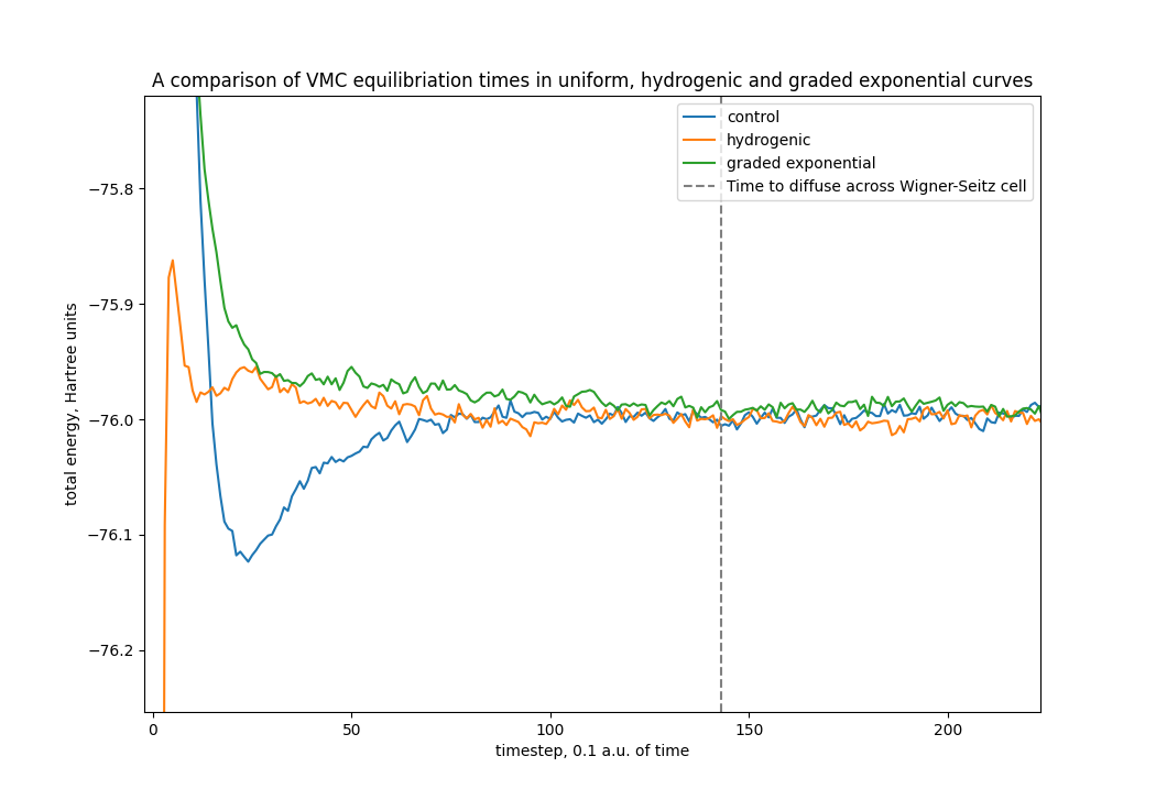
This graph nicely summarises most of my work. Here we can see that the hydrogenic and graded exponential curves converge slightly faster upon the correct value. Note that the dashed grey line simply marks the amount of time it ought to take for the simulation to "explore" the entire system. Typically simulations will converge upon the mean at around this time.
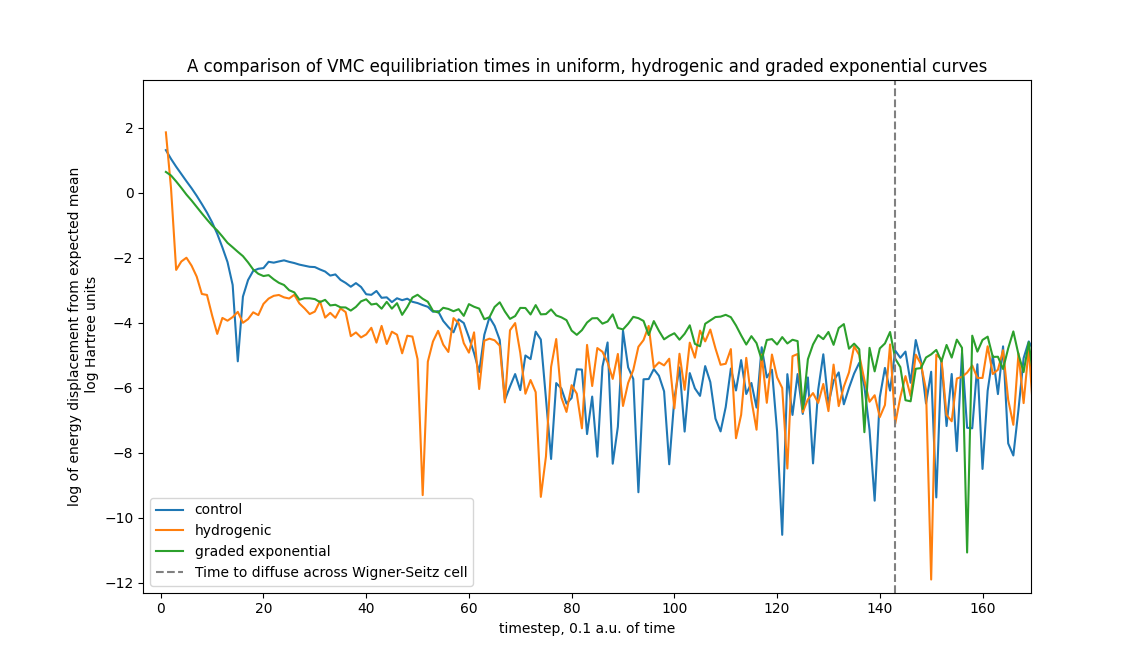
This graph displays the same data as the previous one, but the y-axis displays the natural log of the displacement from the total energy. This means that the lower a result is, the closer it is to the target value.
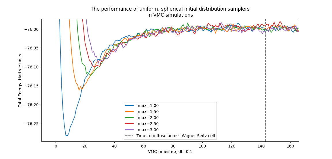
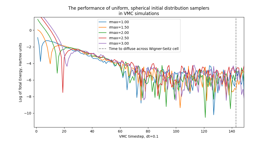
This graph, and the one below, compare the time to equilibriation of five different maximum radii in the control algorithm. As can be seen, changing the radii only affects the first handful of iterations, after around step 30 they all converge at roughly the same rate.
For further reading, please see the following sources:
Foulkes WMC, Mitas L, Needs RJ, Rajagopal G. Quantum Monte Carlo simulations of
solids. Rev Mod Phys. 2001 Jan;73:33–83. Available from: https://link.aps.org/
doi/10.1103/RevModPhys.73.33.
- Generally a good introduction to QMC methods for those with a background in physics.
Needs RJ, Towler MD, Drummond ND, R ́ıos PL. Continuum variational and diffusion
quantum Monte Carlo calculations. 2009 dec;22(2):023201. Available from: https:
//doi.org/10.1088/0953-8984/22/2/023201.
- A source describing the methodology of QMC calculations in great detail. Written by the authors of CASINO, the QMC software I have used.
Metropolis N. The Beginning of the Monte Carlo Method. Los Alamos Science.
1987;15:125–130. Available from: https://la-science.lanl.gov/lascience15.
shtml.
- A history of Monte Carlo simulations, which I found quite an accessible read.
Simas AM, Sagar RP, Ku ACT, Smith Jr VH. The radial charge distribution and the
shell structure of atoms and ions. Canadian Journal of Chemistry. 1988;66(8):1923–
1930. Available from: https://doi.org/10.1139/v88-310.
- A paper on radial charge density functions around atoms, which I used as inspiration for my algorithms.
Slide 1 image (max 2mb)
Slide 1 video (YouTube/Vimeo embed code)
Image 1 Caption
Slide 2 image (max 2mb)
Slide 2 video (YouTube/Vimeo embed code)
Image 2 Caption
Slide 3 image (max 2mb)
Slide 3 video (YouTube/Vimeo embed code)
Image 3 Caption
Slide 4 image (max 2mb)
Slide 4 video (YouTube/Vimeo embed code)
Image 4 Caption
Slide 5 image (max 2mb)
Slide 5 video (YouTube/Vimeo embed code)
Image 5 Caption
Slide 6 image (max 2mb)
Slide 6 video (YouTube/Vimeo embed code)
Image 6 Caption
Slide 7 image (max 2mb)
Slide 7 video (YouTube/Vimeo embed code)
Image 7 Caption
Slide 8 image (max 2mb)
Slide 8 video (YouTube/Vimeo embed code)
Image 8 Caption
Slide 9 image (max 2mb)
Slide 9 video (YouTube/Vimeo embed code)
Image 9 Caption
Slide 10 image (max 2mb)
Slide 20 video (YouTube/Vimeo embed code)
Image 10 Caption
Caption font
Text
Image (max size: 2mb)
Or drag a symbol into the upload area


Image description/alt-tag
Image caption
Image link
Rollover Image (max size: 2mb)
Or drag a symbol into the upload area
Border colour
Rotate
Skew (x-axis)
Skew (y-axis)
Image (max size: 2mb)
Or drag a symbol into the upload area
Image description/alt-tag
Image caption
Image link
Rollover Image (max size: 2mb)
Or drag a symbol into the upload area
Border colour
Rotate
Skew (x-axis)
Skew (y-axis)
Image (max size: 2mb)
Or drag a symbol into the upload area
Image description/alt-tag
Image caption
Image link
Rollover Image (max size: 2mb)
Or drag a symbol into the upload area
Border colour
Rotate
Skew (x-axis)
Skew (y-axis)
Image (max size: 2mb)
Or drag a symbol into the upload area
Image description/alt-tag
Image caption
Image link
Rollover Image (max size: 2mb)
Or drag a symbol into the upload area
Border colour
Rotate
Skew (x-axis)
Skew (y-axis)
Image (max size: 2mb)
Or drag a symbol into the upload area
Image description/alt-tag
Image caption
Image link
Rollover Image (max size: 2mb)
Or drag a symbol into the upload area
Border colour
Rotate
Skew (x-axis)
Skew (y-axis)