Brandon Tupou
Despite global use since its approval in the clinic over 60 years ago, warfarin remains a difficult anticoagulant to dose correctly. Significant interindividual variability has motivated efforts to personalise warfarin treatment that has focussed on using genetic and clinical factors to optimise warfarin dosage. However, the consensus on whether genotype/clinical-guided algorithms improve anticoagulant therapy is debated. Therefore, this project aims to investigate algorithms developed from control theory by adopting a black-box system identification approach. Namely, the classical PID (proportional-integral-derivative) and PIP-LQ (proportional-integral-plus linear quadratic) controllers are investigated. The dataset analysed contains records of 303 patients describing their INR (international normalised ratio) and corresponding dose adjustment over 14 clinical visits. The control systems are simulated in MATLAB & Simulink and are assessed against performance criteria: stability, setpoint tracking, robustness, and safety. Simulation results concluded that the PIP-LQ controller outperformed the simple PID controller against all performance metrics. These findings indicate the potential application of control systems in current warfarin management and other medical regimes. In conclusion, this project demonstrates that genotype-guided treatment is not essential to optimise warfarin treatment and that the PIP-LQ controller is robust to external disturbances and uncertainties.

Brandon Tupou
Setting the scene
What is warfarin?
‣ Warfarin is an anticoagulant (a.k.a blood thinners) taken daily by millions of people worldwide.
‣ It is commonly prescribed to patients with a history of strokes/heart attacks caused by a blood clot, or by people with mechanical heart valves [1].
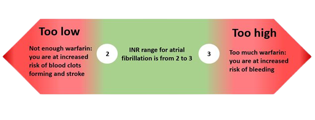
‣ Patients taking warfarin regularly visit their clinician to get their blood clotting speed measured. This is indicated by a metric called the international normalised ratio (INR) and the goal is to maintain this value within a prescribed range (e.g. between 2 and 3) [2].
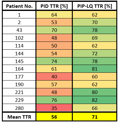
‣ Note: Another metric called time in therapeutic range (TTR) indicates the percentage of INR measurements that are within the desired range.
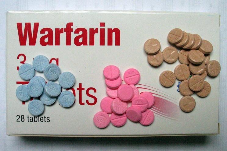
Warfarin tablets come in different colours to indicate their strength in milligrams.
So, what is the problem?
‣ Warfarin is notoriously difficult to dose correctly. Patient safety is the number one priority and getting the dose incorrect can be catastrophic [3] [4] [5].
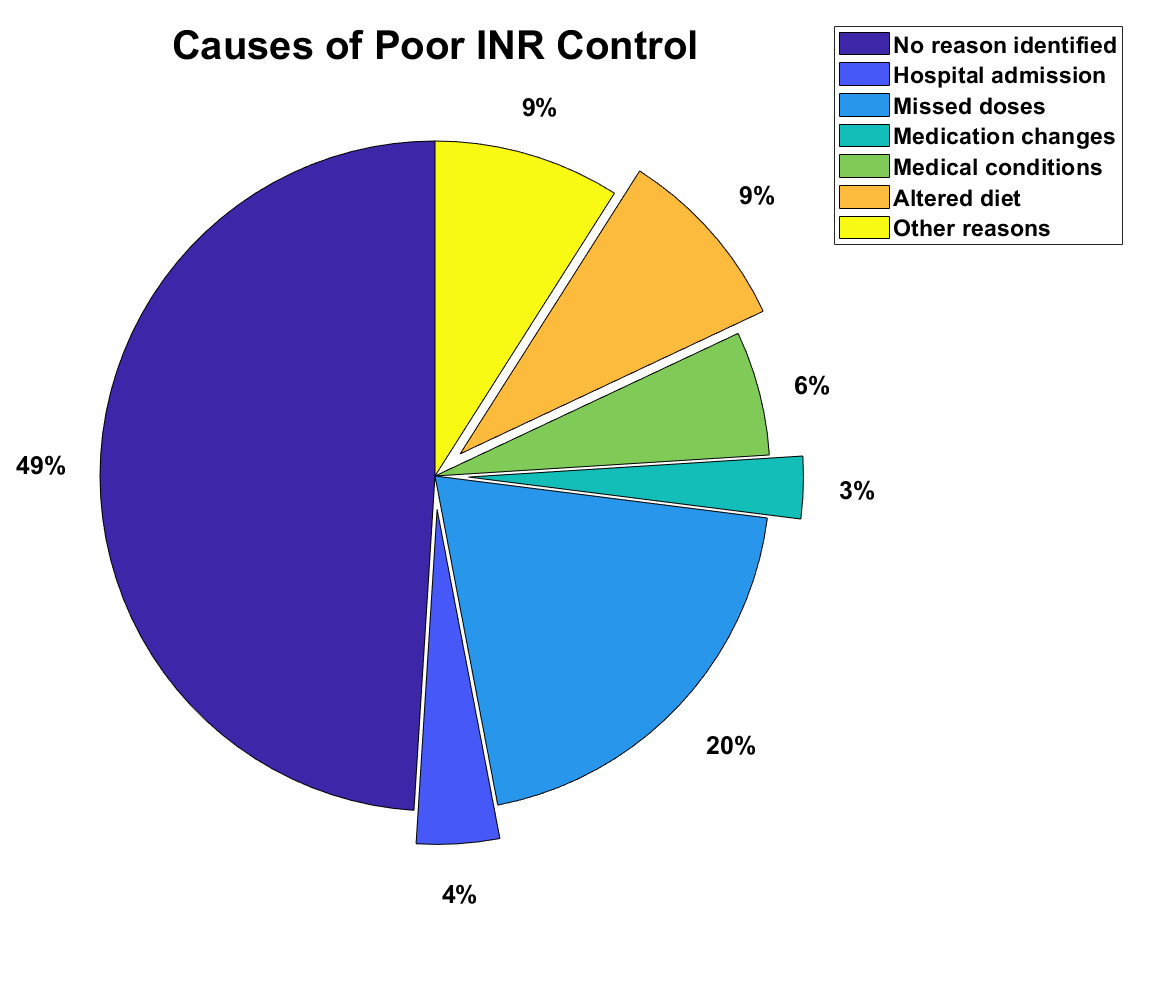
‣ This is because warfarin dynamics are influenced by many genetic and environmental factors (e.g. diet, other interacting drugs) [6] [7]. Furthermore, patients sometimes manifest erratic or unstable INR responses for no particular reason (see pie chart).
‣ Therefore, the challenge is to determine the lowest dose possible that keeps their INR within desired values.
Project aims and methods
Project Aim
This project aims to investigate control algorithms applied to warfarin dose optimisation. These algorithms are developed from the field of control theory. Two types of controllers are investigated:
‣ The classical PID (proportional-integral-derivative) controller is investigated because it has been used widely in engineering for decades for its design simplicity and robustness.
‣ The modern PIP-LQ (proportional-integral-plus linear quadratic) controller is investigated because of its novel design flexibility (chapter 5-6 [8]).
Controllers could be powerful in this biomedical context because they can handle uncertainty (e.g. the random INR fluctuations commonly observed) and can drive a system into its desired state (e.g. the target INR range that is between -0.5 and 0.5 for this project).
Tools: MATLAB & Simulink (CAPTAIN Toolbox, Control systems Toolbox) [10].
‣ Note: don't worry about understanding the terminology. What's important is that PID and PIP-LQ are two different algorithms that do some maths to determine the best dose.
1. Modelling
A mathematical model describing each patient's response dynamics to warfarin is derived using their response history data. This modelling approach is called black-box system identification.
2. Controller Design
Controllers can then be personally designed and tuned to each patient that are driven by the goal to maintain their INR between -0.5 and 0.5 by selecting appropriate doses.

3. Simulation
Finally, each control algorithm is assessed against various performance criteria to assess their robustness (to modelling errors), stability (to random INR fluactions) and setpoint tracking (TTR).

Note: the patient's INR is not measured continuously in real time, rather in discrete intervals with a period of days or weeks between measurements. This is because warfarin does not act instantaneously so we need to wait to see the effects of the drug. The controller takes the INR measurement of that patient at that time to calculate a new dose (if required).
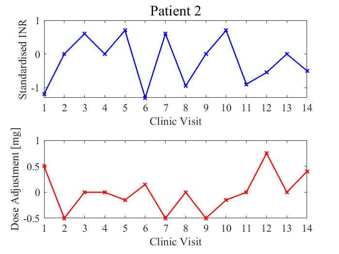
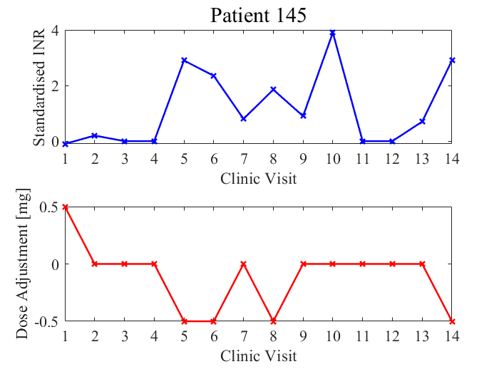
These plots are example patient data used to derive the models. Patient 2 is unstable since their INR measurements fluctuate erratically. Patient 2 TTR = 36% (number of INR values within target range/total number of clinic visits = 3/14 = 36%).
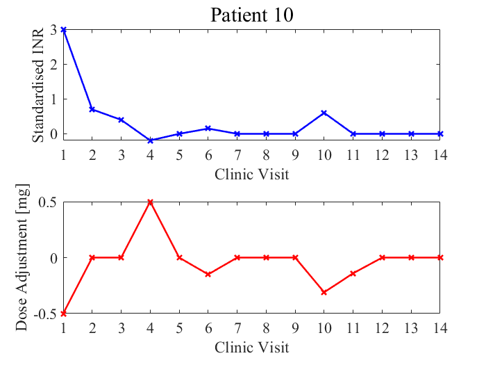
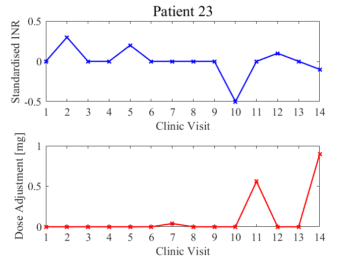
These patients exhibit stable responses. Their INR measurements do not fluctuate erratically and remain within the target INR range (for the most part). Patient 10 TTR = 79% (11/14), patient 23 TTR = 100%.
Results and analysis
Stability and setpoint tracking
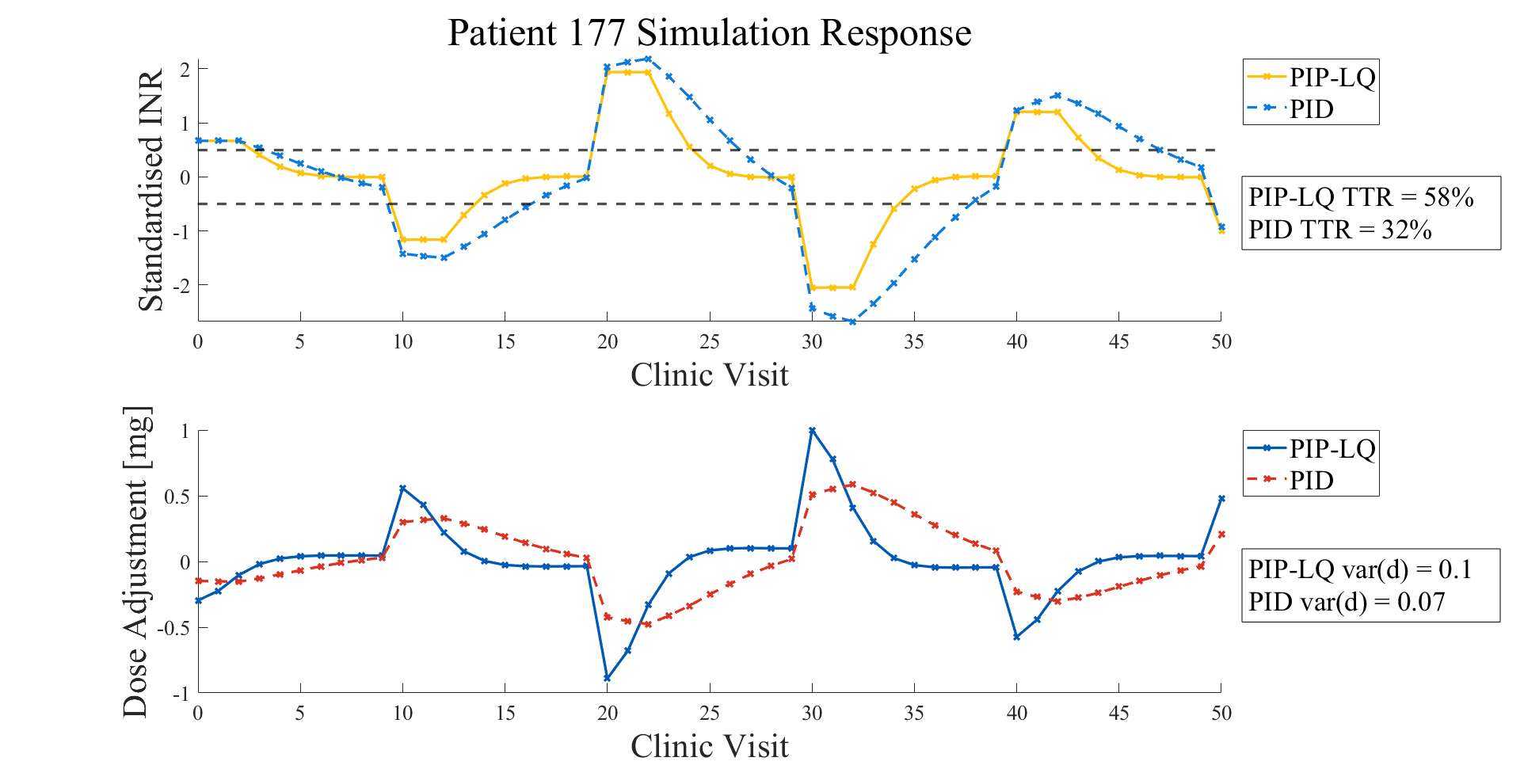
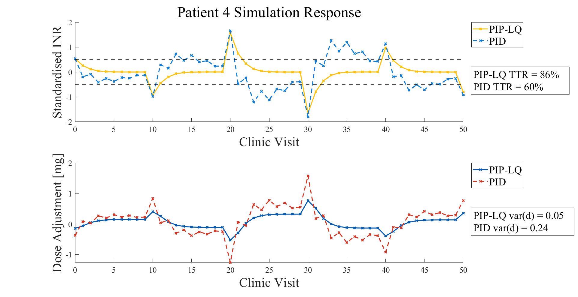
Notice that the PIP-LQ controller produces smaller overshoot (peaks) in the INR compared to the PID controller. Hover to see another example.
Robustness
‣ The control algorithms will always be slightly misdesigned in practice because of modelling inaccuracies (since we design the controllers based on these inaccurate models).
‣ The performance of the controllers under these statistical uncertainties is evaluated through a sensitivity analysis. A Monte Carlo study is employed to assess the performance of the controllers under these model mismatch conditions.
‣ Both controllers show similar robustness characteristics to model mismatch.
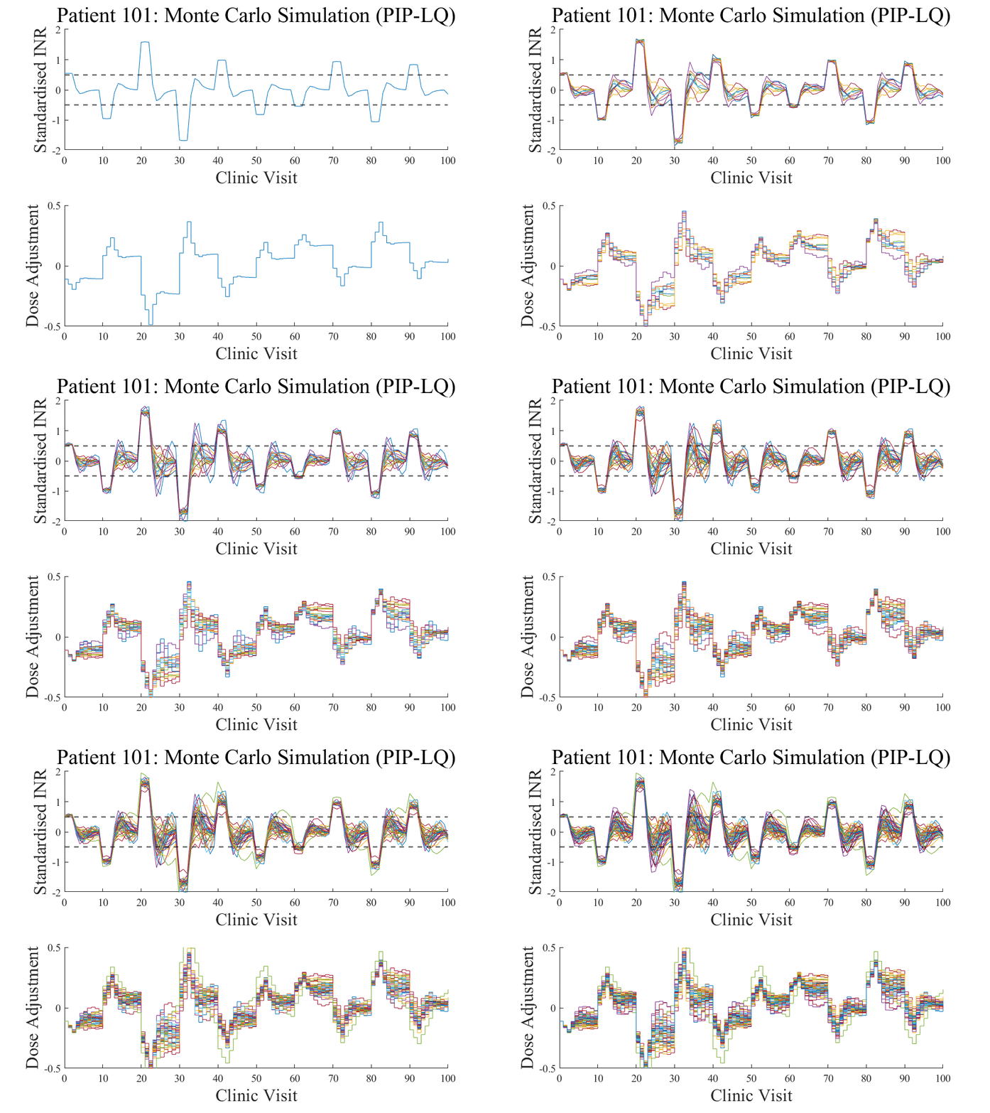
Each response profile is a simulation where the model used by the controller is slightly 'mismatched' to the actual patient's response dynamics to warfarin. Only 50 iterations are shown here but usually Monte Carlo methods involve hundreds or thousands of samples.
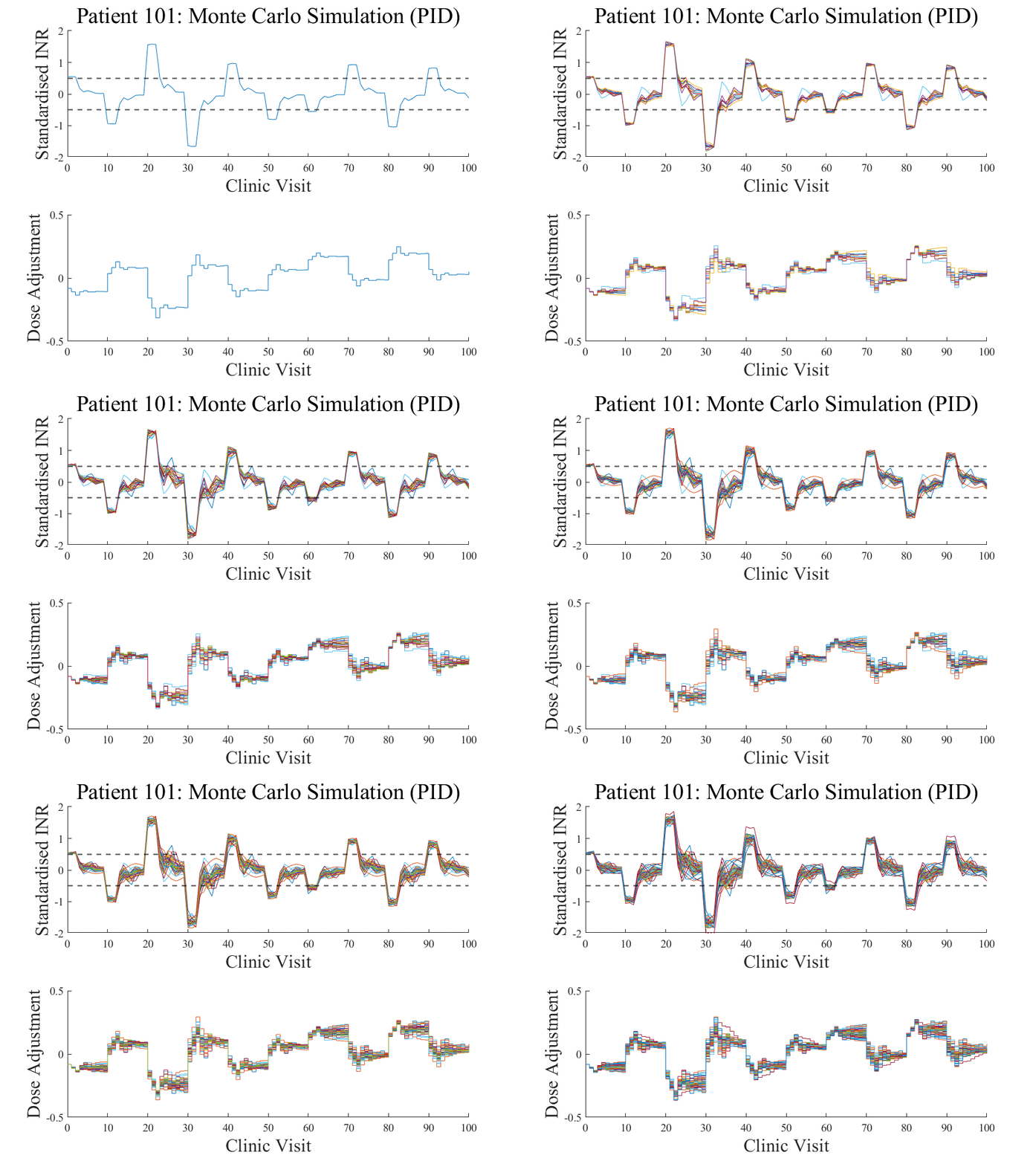
Monte Carlo simulations involve random repeated sampling. The level of 'randomness' is high in this study because of the stochastic and multivariate nature in response to warfarin.
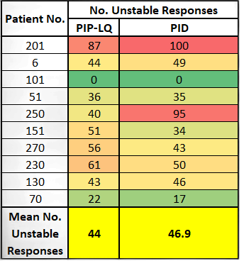
Monte Carlo simulation results for a random sample of 10 patients. Ideally, there should be no unstable responses, but the statistical uncertainty for this research problem is very high.
Safety
‣ The magnitude and profile of the dose adjustments is also important to assess. Making adjustments that oscillate/jump up and down frequently can be dangerous. We assess this by taking the variance of the control dose decisions (var(d)).
‣ Dose variance for the PIP-LQ is smaller, thus makes safer dose changes than the PID control actions.
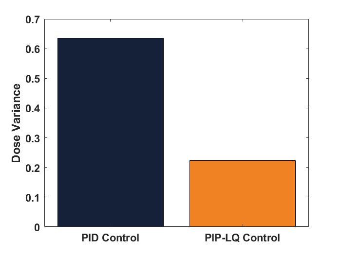
Smaller dose variance = less aggressive (and safer) treatment.
Conclusions
Summary of results
Both controllers show similar robustness characteristics to parametric uncertainty. However, the PIP-LQ controller demonstrates superior handling of INR disturbances compared to the PID controller. Furthermore, the PIP-LQ controller produces smoother dose adjustments compared to the PID algorithm which is safer from a medical perspective.
Despite practical validation with patients, the PIP-LQ controller shows potential for integration in current warfarin management regimes. These control systems could help augment/guide the dose decision process for doctors, leading to safer data-driven anticoagulant treatment. However, trust from medical practitioners must advance to realise this.
Final remarks
Future work could explore multivariate PIP control where patient features, such as age or genotype, are considered. Other medical applications of the PIP-LQ control system include insulin control for diabetes, chemotherapy and real-time patient monitoring systems.
As the amount and diversity of data increases, technologies such as machine learning and control systems will become stronger, especially in biomedical contexts. Big data will not only allow for personalised medicine but enhanced measures for disease prediction and prevention (P4 medicine). The ability to make clinical decisions driven by individual patient data is more powerful than the naive approach of making medical decisions based on population averages.

Thank you to my supervisor Prof. C. James Taylor for their support and guidance. Prof. Taylor is a developer of the CAPTAIN toolbox for MATLAB that has been used extensively in this project [9] [10] . He also developed the PIP control algorithm that you can learn more about from his book 'True Digital Control' [8].

|
[1] |
A. E. Rettie and G. Tai, The Pharmocogenomics of Warfarin: closing in on personalised medicine, vol. 11, Molecular Interventions, 2006. |
|
[2] |
P. A. Tiderman, R. Tirimacco, A. S. John and G. W. Roberts, How to manage warfarin therapy, vol. 38, Australian Prescriber, 2015, pp. 44-48. |
|
[3] |
D. K. Wysowski, P. Nourjah and L. Swartz, Bleeding Complications With Warfarin Use: A Prevalent Adverse Effect Resulting in Regulatory Action, vol. 167, Archives of Internal Medicine, 2007, pp. 1414-1419. |
|
[4] |
M. Pirmohamed, Warfarin: almost 60 years old and still causing problems, vol. 62, British Journal of Clinical Pharmacology, 2006, pp. 509-511. |
|
[5] |
S. D. Pokorney, D. N. Simon, L. Thomas, B. J. Gersh, E. M. Hylek, J. P. Piccini and E. D. Peterson, Stability of International Normalized Ratios in Patients Taking Long-term Warfarin Therapy, vol. 316, JAMA, 2016, pp. 661-663. |
|
[6] |
T.-L. Wang, H.-l. Li, W.-Y. Tjong, Q.-S. Chen, G.-S. Wu, H.-T. Zhu, Z.-S. Hou, S. Xu, S.-J. Ma, M. Wu and S. Tai, Genetic factors contribute to patient-specific warfarin dose for Han Chinese, vol. 396, Clinica Chimica Acta, 2008, pp. 76-79. |
|
[7] |
M. D. Caldwell, R. L. Berg, K. Q. Zhang, I. Glurich, J. R. Schmelzer, S. H. Yale, H. J. Vidaillet and J. K. Burmester, Evaluation of Genetic Factors for Warfarin Dose Prediction, vol. 5, Clinical Medicine & Research, 2007, pp. 8-16. |
|
[8] |
J. C. Taylor, P. C. Young and A. Chotai, True Digital Control: Statistical Modelling and Non-Minimal State Space Design, Lancaster: Wiley, 2013. |
|
[9] |
P. Young, The data-based mechanistic approach to the modelling, forecasting and control of environmental systems, vol. 30, Annual Reviews in Control, 2006, pp. 169-182. |
|
[10] |
J. C. Taylor, D. J. Pedregal, P. C. Young and W. Tych, Environmental time series analysis and forecasting with the Captain toolbox, vol. 22, Environment Modelling & Software, 2007, pp. 797-814. |
Slide 1 image (max 2mb)
Slide 1 video (YouTube/Vimeo embed code)
Image 1 Caption
Slide 2 image (max 2mb)
Slide 2 video (YouTube/Vimeo embed code)
Image 2 Caption
Slide 3 image (max 2mb)
Slide 3 video (YouTube/Vimeo embed code)
Image 3 Caption
Slide 4 image (max 2mb)
Slide 4 video (YouTube/Vimeo embed code)
Image 4 Caption
Slide 5 image (max 2mb)
Slide 5 video (YouTube/Vimeo embed code)
Image 5 Caption
Slide 6 image (max 2mb)
Slide 6 video (YouTube/Vimeo embed code)
Image 6 Caption
Slide 7 image (max 2mb)
Slide 7 video (YouTube/Vimeo embed code)
Image 7 Caption
Slide 8 image (max 2mb)
Slide 8 video (YouTube/Vimeo embed code)
Image 8 Caption
Slide 9 image (max 2mb)
Slide 9 video (YouTube/Vimeo embed code)
Image 9 Caption
Slide 10 image (max 2mb)
Slide 20 video (YouTube/Vimeo embed code)
Image 10 Caption
Caption font
Text
Image (max size: 2mb)
Or drag a symbol into the upload area


Image description/alt-tag
Image caption
Image link
Rollover Image (max size: 2mb)
Or drag a symbol into the upload area


Border colour
Rotate
Skew (x-axis)
Skew (y-axis)
Image (max size: 2mb)
Or drag a symbol into the upload area


Image description/alt-tag
Image caption
Image link
Rollover Image (max size: 2mb)
Or drag a symbol into the upload area


Border colour
Rotate
Skew (x-axis)
Skew (y-axis)
Image (max size: 2mb)
Or drag a symbol into the upload area


Image description/alt-tag
Image caption
Image link
Rollover Image (max size: 2mb)
Or drag a symbol into the upload area


Border colour
Rotate
Skew (x-axis)
Skew (y-axis)
Image (max size: 2mb)
Or drag a symbol into the upload area


Image description/alt-tag
Image caption
Image link
Rollover Image (max size: 2mb)
Or drag a symbol into the upload area


Border colour
Rotate
Skew (x-axis)
Skew (y-axis)
Image (max size: 2mb)
Or drag a symbol into the upload area


Image description/alt-tag
Image caption
Image link
Rollover Image (max size: 2mb)
Or drag a symbol into the upload area


Border colour
Rotate
Skew (x-axis)
Skew (y-axis)
Image (max size: 2mb)
Or drag a symbol into the upload area


Image description/alt-tag
Image caption
Image link
Rollover Image (max size: 2mb)
Or drag a symbol into the upload area


Border colour
Rotate
Skew (x-axis)
Skew (y-axis)
Image (max size: 2mb)
Or drag a symbol into the upload area


Image description/alt-tag
Image caption
Image link
Rollover Image (max size: 2mb)
Or drag a symbol into the upload area


Border colour
Rotate
Skew (x-axis)
Skew (y-axis)
Image (max size: 2mb)
Or drag a symbol into the upload area


Image description/alt-tag
Image caption
Image link
Rollover Image (max size: 2mb)
Or drag a symbol into the upload area


Border colour
Rotate
Skew (x-axis)
Skew (y-axis)
Image (max size: 2mb)
Or drag a symbol into the upload area


Image description/alt-tag
Image caption
Image link
Rollover Image (max size: 2mb)
Or drag a symbol into the upload area


Border colour
Rotate
Skew (x-axis)
Skew (y-axis)
Image (max size: 2mb)
Or drag a symbol into the upload area


Image description/alt-tag
Image caption
Image link
Rollover Image (max size: 2mb)
Or drag a symbol into the upload area


Border colour
Rotate
Skew (x-axis)
Skew (y-axis)
Image (max size: 2mb)
Or drag a symbol into the upload area


Image description/alt-tag
Image caption
Image link
Rollover Image (max size: 2mb)
Or drag a symbol into the upload area


Border colour
Rotate
Skew (x-axis)
Skew (y-axis)
Image (max size: 2mb)
Or drag a symbol into the upload area


Image description/alt-tag
Image caption
Image link
Rollover Image (max size: 2mb)
Or drag a symbol into the upload area


Border colour
Rotate
Skew (x-axis)
Skew (y-axis)
Image (max size: 2mb)
Or drag a symbol into the upload area


Image description/alt-tag
Image caption
Image link
Rollover Image (max size: 2mb)
Or drag a symbol into the upload area


Border colour
Rotate
Skew (x-axis)
Skew (y-axis)
Image (max size: 2mb)
Or drag a symbol into the upload area


Image description/alt-tag
Image caption
Image link
Rollover Image (max size: 2mb)
Or drag a symbol into the upload area


Border colour
Rotate
Skew (x-axis)
Skew (y-axis)
Image (max size: 2mb)
Or drag a symbol into the upload area


Image description/alt-tag
Image caption
Image link
Rollover Image (max size: 2mb)
Or drag a symbol into the upload area


Border colour
Rotate
Skew (x-axis)
Skew (y-axis)
Image (max size: 2mb)
Or drag a symbol into the upload area


Image description/alt-tag
Image caption
Image link
Rollover Image (max size: 2mb)
Or drag a symbol into the upload area


Border colour
Rotate
Skew (x-axis)
Skew (y-axis)
Image (max size: 2mb)
Or drag a symbol into the upload area


Image description/alt-tag
Image caption
Image link
Rollover Image (max size: 2mb)
Or drag a symbol into the upload area


Border colour
Rotate
Skew (x-axis)
Skew (y-axis)
Image (max size: 2mb)
Or drag a symbol into the upload area


Image description/alt-tag
Image caption
Image link
Rollover Image (max size: 2mb)
Or drag a symbol into the upload area


Border colour
Rotate
Skew (x-axis)
Skew (y-axis)
