3.5 Properties of $Y\sim \mathrm{EF}$

First, the the moment generating function is

	$𝔼[\exp \{sY\}]$	$=$	${\displaystyle {\int }_{-\mathrm{\infty }}^{\mathrm{\infty }}}\exp \{sy\}\exp \{\theta y-\kappa (\theta )\}q(y)𝑑y$
		$=$	$\exp \{-\kappa (\theta )\}{\displaystyle {\int }_{-\mathrm{\infty }}^{\mathrm{\infty }}}\exp \{sy+\theta y\}q(y)𝑑y$
		$=$	$\exp \{-\kappa (\theta )\}{𝔼}_q[\exp \{(s+\theta )Y\}]$
		$=$	$\exp \{-\kappa (\theta )\}{M}_q(s+\theta )$
		$=$	$\exp \{-\kappa (\theta )\}\exp \{\log M_q(s+\theta )\}$
		$=$	$\exp \{-\kappa (\theta )\}\exp \{\kappa (s+\theta )\}.$

Taking logs gives the cgf

$K(s)=\log 𝔼[\exp \{sY\}]=\kappa (s+\theta )-\kappa (\theta ),$

where $s$ is such that $s+\theta$ lies in $\mathrm{\Theta }$. When we need to make it clear that $K$ is the cgf of $Y$ then we write $K_Y(s)$.

The corollary to this result are that: apart from the first, the cumulants of $Y\sim f\in \mathrm{EF}(\theta ,q)$ are given by the same function as $Y\sim q$. The mean and variance of $Y$ under $f$ are given by evaluating the derivatives of the cgf evaluated at $s=0$, $K^{\prime }(0)$ and $K^{\prime \prime }(0)$. Now

	$K^{\prime }(s)={\displaystyle \frac{d}{ds}}K(s)$	$=$	${\displaystyle \frac{d}{ds}}\kappa (s+\theta )$
		$=$	${\displaystyle \frac{d\kappa (s+\theta )}{d(s+\theta )}}{\displaystyle \frac{d(s+\theta )}{ds}}\mathit{\hspace{1em}\hspace{0.25em}}[\mathrm{ChainRule}]$
		$=$	${\kappa }^{\prime }(s+\theta )\times 1\mathit{\hspace{1em}}\mathrm{so}$
	$K^{\prime }(0)$	$=$	${\kappa }^{\prime }(\theta )$
		$=$	${\kappa }_{\theta }(\theta ).$

Furthermore

	$K^{\prime \prime }(s)$	$=$	${\kappa }^{\prime \prime }(s+\theta )\mathit{\hspace{1em}}\mathrm{so}$
	$K^{\prime \prime }(0)$	$=$	${\kappa }^{\prime \prime }(\theta )$
		$=$	${\kappa }_{\theta \theta }(\theta ).$

Using the properties of a cgf that $K^{\prime }(0)$ and $K^{\prime \prime }(0)$ give the mean and variance, we have

$𝔼[Y]={\kappa }_{\theta }(\theta )\mathit{\hspace{1em}}\mathrm{and}\mathit{\hspace{1em}}\mathrm{var}(Y)={\kappa }_{\theta \theta }(\theta ).$

The subscript denotes derivatives with respect to $\theta$. We need this notation to the more usual ${\kappa }^{\prime }(\theta )$ when we change variables and need to keep track.

 
Exercise 3.26
Find the cgf of the Poisson distribution in terms of the canonical parameter, and hence its mean and variance.

 

Recall that if $Y$ is from the exponential family, then the random variable $X$ under the one-to-one transformation $Y=T(X)$ is also a member of the exponential family. If the transform is linear, i.e. $Y=aX+b$, then we can derive the expectation and variance of $X$ from the results above:

$$𝔼[X]=\frac{𝔼[Y]-b}{a}=\frac{{\kappa }_{\theta }(\theta )-b}{a}\mathit{\hspace{1em}}\mathrm{and}\mathit{\hspace{1em}}\mathrm{var}(X)=\frac{\mathrm{var}(Y)}{a^2}=\frac{{\kappa }_{\theta \theta }(\theta )}{a^2}$$

For other non-linear transformations, however, this is not possible as expectations and functions of random variables are not commutable.

Nevertheless, using the relationship between the random variables $X$ and $Y$ we can show that their moment generating functions are related by:

	${𝔼}_Y[\exp \{sY\}]$	$={\displaystyle \int \exp \{sY\}{f}_Y(y|\theta )𝑑y}$
		$={\displaystyle \int }\exp \{sT(x)\}{f}_Y(y=T(x)|\theta ){\displaystyle \frac{dy}{dx}}dx$
		$={\displaystyle \int \exp \{sT(x)\}{f}_X(x|\theta )𝑑x}$
		$={𝔼}_X[\exp \{sT(X)\}]$

We can therefore define the moment generating function for the sufficient statistic $T(X)$ by utilising our previous findings:

$$M_{T(X)}(s)={𝔼}_X[\exp \{sT(X)\}]={𝔼}_Y[\exp \{sY\}]=\exp \{\kappa (s+\theta )-\kappa (\theta )\},$$

and too the cgf for the sufficient statistic:

$$K_{T(X)}(s)=\kappa (s+\theta )-\kappa (\theta )$$

Following the same argument as previously, we can therefore define the expectation and variance of $T(X)$ as:

$$𝔼[T(X)]={\kappa }_{\theta }(\theta )\mathit{\hspace{1em}}\mathrm{and}\mathit{\hspace{1em}}\mathrm{var}(T(X))={\kappa }_{\theta \theta }(\theta ).$$

 
Exercise 3.27
For the random variable $X\sim \mathrm{Gamma}(\alpha ,1)$, find an expression for $𝔼[\log X]$ and $\mathrm{var}(\log X)$.

 

First, define the log-likelihood function for the canonical parameter $\theta$, based on a single observation $y$, by:

$\mathrm{\ell }(\theta )=\log f(y|\theta ).$

Take care: the log-likelihood is also calculated as a function of the mean parameter $\mu$. We are about to show that the relationship between $\mu$ and $\theta$ is invertible so that the log-likelihoods are consistent. When we need to make $y$ explicit we write $\mathrm{\ell }(\theta ;y)$.

Denote its derivatives of the log-likelihood with respect to $\theta$ by:

${\mathrm{\ell }}_{\theta }={\displaystyle \frac{d\mathrm{\ell }(\theta )}{d\theta }}\mathit{\hspace{1em}}\mathrm{and}\mathit{\hspace{1em}}{\mathrm{\ell }}_{\theta \theta }={\displaystyle \frac{d^2\mathrm{\ell }(\theta )}{d{\theta }^2}}.$

Mean and variance of the score

In principle, both the score function and the observed information function are functions of the canonical parameter $\theta$ and the observation $y$. Taking the expected value of the score function over $Y$ results in:

$${𝔼}_Y[{\mathrm{\ell }}_{\theta }(\theta ;Y)]=0$$

PROOF:

	${𝔼}_Y[{\mathrm{\ell }}_{\theta }(\theta ;Y)]$	$={\displaystyle \int {\mathrm{\ell }}_{\theta }(\theta ;y)f(y|\theta )𝑑y}$
		$={\displaystyle \int \frac{d}{d\theta }\left\{\log f(y|\theta )\right\}f(y|\theta )𝑑y}$
		$={\displaystyle \int \frac{\frac{d}{d\theta }f(y|\theta )}{f(y|\theta )}f(y|\theta )𝑑y}$
		$={\displaystyle \int \frac{d}{d\theta }f(y|\theta )𝑑y}$
		$={\displaystyle \frac{d}{d\theta }}{\displaystyle \int f(y|\theta )𝑑y}$
		$={\displaystyle \frac{d}{d\theta }}\{1\}=0.$

The variance of the score function is:

$${\mathrm{var}}_Y({\mathrm{\ell }}_{\theta }(\theta ;Y))=-{𝔼}_Y[{\mathrm{\ell }}_{\theta \theta }(\theta ;Y)]$$

PROOF

	${\mathrm{var}}_Y({\mathrm{\ell }}_{\theta }(\theta ;Y))+{𝔼}_Y[{\mathrm{\ell }}_{\theta \theta }(\theta ;Y)]$
	$\mathrm{ }\mathit{\hspace{1em}\hspace{0.5em}}={𝔼}_Y[{\mathrm{\ell }}_{\theta }{(\theta ;Y)}^2]-{𝔼}_Y{[{\mathrm{\ell }}_{\theta }(\theta ;Y)]}^2+{𝔼}_Y[{\mathrm{\ell }}_{\theta \theta }(\theta ;Y)]$
	$\mathrm{ }\mathit{\hspace{1em}\hspace{0.5em}}={𝔼}_Y[{\mathrm{\ell }}_{\theta }{(\theta ;Y)}^2+{\mathrm{\ell }}_{\theta \theta }(\theta ;Y)]$
	$\mathrm{ }\mathit{\hspace{1em}\hspace{0.5em}}={\displaystyle \int }[{\left\{{\displaystyle \frac{d}{d\theta }}\log f(y|\theta )\right\}}^2+{\displaystyle \frac{d{}^2}{d{\theta }^2}}\log f(y|\theta )]f(y|\theta )dy$
	$\mathrm{ }\mathit{\hspace{1em}\hspace{0.5em}}={\displaystyle \int }[\left\{{\displaystyle \frac{d}{d\theta }}\log f(y|\theta )\right\}{\displaystyle \frac{\frac{d}{d\theta }f(y|\theta )}{f(y|\theta )}}+{\displaystyle \frac{d{}^2}{d{\theta }^2}}\log f(y|\theta )]f(y|\theta )dy$

	$\mathrm{ }={\displaystyle \int \frac{d}{d\theta }\log f(y|\theta )\times \frac{d}{d\theta }f(y|\theta )}+{\displaystyle \frac{d{}^2}{d{\theta }^2}}\log f(y|\theta )\times f(y|\theta )dy\mathit{\hspace{1em}\hspace{0.25em}}[\mathrm{ByProductRule}]$
	$\mathrm{ }={\displaystyle \int \frac{d}{d\theta }\left[\frac{d}{d\theta }\log f(y|\theta )\times f(y|\theta )\right]𝑑y}$
	$\mathrm{ }={\displaystyle \int \frac{d}{d\theta }\left[\frac{\frac{d}{d\theta }f(y|\theta )}{f(y|\theta )}f(y|\theta )\right]𝑑y}$
	$\mathrm{ }={\displaystyle \int \frac{d{}^2}{d{\theta }^2}f(y|\theta )𝑑y}$
	$\mathrm{ }={\displaystyle \frac{d{}^2}{d{\theta }^2}}{\displaystyle \int f(y|\theta )𝑑y}={\displaystyle \frac{d{}^2}{d{\theta }^2}}[1]=0$

This is the big news! We now specialize these results to EF distributions. The log-likelihood function, the score function and the curvature function, for a single observation, are

	$\mathrm{\ell }(\theta )$	$=$	$\theta y-\kappa (\theta )+\log q(y)$
	${\mathrm{\ell }}_{\theta }(\theta )$	$=$	$y-{\kappa }_{\theta }(\theta )$
	${\mathrm{\ell }}_{\theta \theta }(\theta )$	$=$	$-{\kappa }_{\theta \theta }(\theta ).$

The score is linear in $y$ and the observed information is constant with respect to $y$. Hence the latter is identical to the Fisher or expected information.

This provides us with an alternative way to find the first two moments of $Y$. From above, the expectation of $Y$ is:

$${𝔼}_Y[Y]={𝔼}_Y[{\mathrm{\ell }}_{\theta }(\theta ;Y)+{\kappa }_{\theta }(\theta )]={𝔼}_Y[{\mathrm{\ell }}_{\theta }(\theta ;Y)]+{\kappa }_{\theta }(\theta )={\kappa }_{\theta }(\theta )$$

and the variance of $Y$ is:

$${\mathrm{var}}_Y(Y)={\mathrm{var}}_Y({\mathrm{\ell }}_{\theta }(\theta ;Y)+{\kappa }_{\theta }(\theta ))={\mathrm{var}}_Y({\mathrm{\ell }}_{\theta }(\theta ;Y))=-{𝔼}_Y[{\mathrm{\ell }}_{\theta \theta }(\theta ;Y)]={\kappa }_{\theta \theta }(\theta )$$

A sufficient condition for a function to be strictly convex is that its second derivative be strictly positive. Hence the function $\kappa (\theta )$ is strictly convex on $\mathrm{\Theta }$, because the second derivative of $\kappa$ is ${\kappa }_{\theta \theta }(\theta )=\mathrm{var}(Y)$ which is always positive.

Consider a set of independent and identically distributed random variables $y_1,\mathrm{\dots },y_n$ from some random variable belonging to the exponential family with pmf/pdf:

$$f(y_i|\theta )=q(y_i)\exp \{y_i\theta -\kappa (\theta )\}\mathit{\hspace{1em}}\text{for}i=1,\mathrm{\dots },n.$$

The log-likelihood of the canonical parameter for all realisations is the summation of all log-likelihood contributions from each $y_i$:

	$\mathrm{\ell }(\theta )$	$={\displaystyle \sum _{i=1}^n}\mathrm{\ell }(\theta |y_i)$
		$={\displaystyle \sum _{i=1}^n}\left\{\theta y_i-\kappa (\theta )+\log q(y_i)\right\}$
		$=\theta {\displaystyle \sum _{i=1}^n}{y}_i-n\kappa (\theta )+{\displaystyle \sum _{i=1}^n}\log q(y_i)$

Taking derivatives obtains the score and curvature functions:

	${\mathrm{\ell }}_{\theta }(\theta )$	$={\displaystyle \sum _{i=1}^n}{y}_i-n{\kappa }_{\theta }(\theta )$
	${\mathrm{\ell }}_{\theta \theta }(\theta )$	$=-n{\kappa }_{\theta \theta }(\theta )$

where ${\kappa }_{\theta }(\theta )$ and ${\kappa }_{\theta \theta }(\theta )$ respectively denote the first and second derivatives of the function $\kappa (\theta )$.

The maximum likelihood estimate (MLE) for the canonical parameter, $\widehat{\theta }$, is evaluated by finding the roots of the score function:

$$0=\sum _{i=1}^n{y}_i-n{\kappa }_{\theta }(\widehat{\theta })\mathit{\hspace{1em}}\iff \mathit{\hspace{1em}}{\kappa }_{\theta }(\widehat{\theta })=\frac{1}{n}\sum _{i=1}^n{y}_i$$

An analytical definition of the MLE is found by deriving the inverse of the derivative function ${\kappa }_{\theta }(\theta )$. If an analytical solution does not exist, then the MLE can be determined using a numerical algorithm such as Newton-Raphson.

The observed information for the canonical parameter evaluated at some value ${\theta }^{*}$ is

$$I_O({\theta }^{*})=-{\mathrm{\ell }}_{\theta \theta }(\theta ={\theta }^{*})=n{\kappa }_{\theta \theta }(\theta ={\theta }^{*})$$

Note that the observed information for the canonical parameter of a pmf/pdf which belongs to the exponential family does not depend on the value of the realisations, but only on how many realisations there are. It follows that the expected information at ${\theta }^{*}$ is:

$$I_E({\theta }^{*})={𝔼}_Y[I_O({\theta }^{*})]={𝔼}_Y[n{\kappa }_{\theta \theta }({\theta }^{*})]=n{\kappa }_{\theta \theta }({\theta }^{*}).$$

In many instances, the observed and expected information is evaluated at the MLE, ${\theta }^{*}=\widehat{\theta }$.

 
Exercise 3.28
Recall that the $\mathrm{Poisson}(\lambda )$ distribution belongs to the exponential family with canonical parameter $\theta =\log (\lambda )$ and:

$$\kappa (\theta )=\exp \{\theta \}-1.$$

Find the MLE of the canonical parameter $\widehat{\theta }$ for independent and identically distributed realisations $y_1,\mathrm{\dots },y_n$ from the Poisson distribution. Also derive an expression for the expected information at the MLE.

 

A central role in EF theory is played by the function that computes the moment parameter $\mu$ from the value of the canonical parameter $\theta$.

The mean function is sometimes known as the mean value function. The moment parameter space $\mathrm{\Omega }$ is the range space of the mapping from $\theta$ to $\mu$.

The mean function plays an important part in the theory. For example, maximum likelihood estimates of $\theta$ turn out to be solutions to the equation $m(\theta )=y$.

 
Exercise 3.29
Find the mean function for the Poisson distribution, in terms of the canonical parameter, and its inverse.

 

 
Exercise 3.30
Find the cgf of $\mathrm{Binom}(k,1/2)$.

Find the mean function for the binomial distribution $\mathrm{Binom}(k,\pi )$ with generated by exponentially tilting $\mathrm{Binom}(k,1/2)$.

 

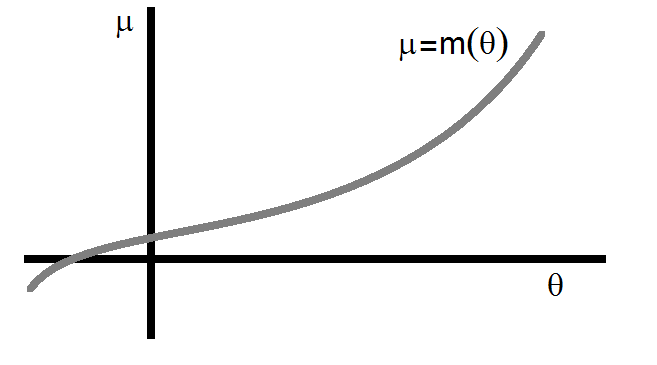
From the discussion of $\kappa$ it follows that $m$ too, is continuous and differentiable on the interior of $\mathrm{\Theta }$. The first derivative of $m(\theta )$ is

$m_{\theta }={\kappa }_{\theta \theta }=\mathrm{var}(Y)$

so that $m_{\theta }(\theta )>0$ for all $\theta$. Hence $m(\theta )$ is a strictly increasing function of $\theta$ as portrayed in the diagram.

Consequently the mapping from $\theta$ to $\mu$ is invertible. Hence there is a function $m^{-1}$ going from $\mathrm{\Omega }$ to $\mathrm{\Theta }$ such that

$\theta =m^{-1}(\mu ).$

By the inverse function rule of differentiation

${\displaystyle \frac{d\theta }{d\mu }}={\left({\displaystyle \frac{d\mu }{d\theta }}\right)}^{-1}={\displaystyle \frac{1}{m_{\theta }}}={\displaystyle \frac{1}{\mathrm{var}(Y)}}>0.$

The inverse mean function $m^{-1}$ plays the role of the link function $g$ when the canonical parameter is chosen to be the linear predictor.

ML from a single observation

Recall that the score function based on a single observation, and obtained by differentiating the log-likelihood as a function of the canonical parameter $\theta$, is

${\mathrm{\ell }}_{\theta }(\theta )=y-{\kappa }_{\theta }(\theta )=y-m(\theta ),$

using the definition of the mean function $m$. Hence if $\theta$ is a free parameter then its ML estimate satisfies

$0=y-m(\widehat{\theta })\iff \widehat{\theta }=m^{-1}(y),$

as $m$ is invertible. Finally as $\mu =m(\theta )$, $\widehat{\mu }=m(\widehat{\theta })$,

$\widehat{\mu }$

$=$

$y.$

Equating observation with theoretical moments is a general feature of the likelihood equations in GLMs.

 
Exercise 3.31
Derive the MLE for the canonical parameter for a single measurement, $y$, of a Poisson random variable.

 

 
Exercise 3.32
Find an expression for the MLE of the canonical parameter $\widehat{\theta }$ given a single observation, $x$, from $X\sim \mathrm{Gamma}(\alpha ,1)$.

 

The relationship of the variance of $Y$ to the mean of $Y$ characterizes linear EF distributions. We want to compute $\mathrm{var}(Y)$ in terms of the moment parameter $\mu =𝔼[Y]$.

This definition expresses the variance in terms of the canonical parameter $\theta$. Since

$v(\mu )={\kappa }_{\theta \theta }(\theta )=m_{\theta }(\theta ).$

Substitute for the canonical parameter $\theta$ in terms of $\mu$ to get

$v(\mu )=\mathrm{var}(Y)=m_{\theta }(\theta )=m_{\theta }[m^{-1}(\mu )].$

 
Exercise 3.33
Find the variance function for the Poisson distribution.

 

 
Exercise 3.34
Find the variance function for the Exponential distribution.