Multiple linear regression follows exactly the same concept as simple linear regression, except that the expected value of the response variable may depend on more than one explanatory variable.

• The multiple linear regression model has a very similar definition to the simple linear regression model, except that

  1. missingi.

     Each individual has a single response variable $Y_i$, but a missingmissingvector

  of explanatory variables $(x_{i,1},\mathrm{\dots },x_{i,p})$. The number of explanatory variables is denoted by $p$.

• There are $p$ regression coefficients ${\beta }_1,{\beta }_2,\mathrm{\dots },{\beta }_p$, where ${\beta }_j$ describes the effect of the $j$-th explanatory variable on the expected value of the response.

An informal definition of the multiple linear model is {mdframed}

• –

  $Y_i\sim \mathrm{N}({\sum }_{j=1}^p{\beta }_j{x}_{i,j},{\sigma }^2)$, $i=1,\mathrm{\dots },n$;

• –

  $Y_1,\mathrm{\dots },Y_n$ are independent.

Later in the course it will be useful to write our models using the following matrix notation.

• The response vector $Y={(Y_1,\mathrm{\dots },Y_n)}^{\mathrm{missing}}\prime$

  • The design matrix $X$ is an $n\times p$ matrix whose columns correspond to explanatory variables and whose rows correspond to subjects. That is $X_{\mathrm{missing}}i,j$ denotes the value of the $j$-th explanatory variable for individual $i$. If an intercept term is included, then the first column of $X$ is a column of 1’s.

    • The residual vector $ϵ={({ϵ}_1,\mathrm{\dots },{ϵ}_n)}^{\mathrm{missing}}\prime$

      • The $p\times 1$ vector of coefficients is missing$\beta ={({\beta }_1,\mathrm{\dots },{\beta }_p)}^{\mathrm{missing}}\prime$

      Then we can write the multiple linear regression model as follows,

      • 1

        $Y=X\beta +ϵ$ where $ϵ\sim {\mathrm{MVN}}_n(0,{\sigma }^{2}I)$ and $I$ is the $n\times n$ identity matrix.

      • 2

        Informally, $Y\sim {\mathrm{MVN}}_n(X\beta ,{\sigma }^{2}I)$.

      For the remainder of the course we will not distinguish between simple and multiple linear regression, since the former is a special case of the latter. Instead we refer to linear regression.

      Remark.

      Because of the normality assumption on the residuals the full title of the model is the normal linear regression model.

      Response variables

      From the informal definition of the linear regression model, the response variable $Y_i$ should be continuous and follow a normal distribution. It only makes sense to apply a linear regression model to data for which the response variable satisfies these criteria.

      The assumption of normality can be verified with a normal QQ plot. If the response if continuous and non-normal, a transformation may be used to transform to normality. For example, we might take the log or square root of the responses.

      Math333 will introduce the concept of the generalised linear model, in which the normality assumption is relaxed to cover a wide family of distributions, including the Poisson and binomial.

      Factors

      Explanatory variables may be continuous or discrete, qualitative or quantitative.

      Definition.

      • 1

        A covariate is a quantitative explanatory variable.
        

      • 2

        A factor is a qualitative explanatory variable. The possible values for the factor are called levels. For example, gender is a two-level factor with two levels: male and female.

      Factors are represented by indicator variables in a linear regression model. For a $p$-level factor, $p$ indicator variables are created. For individual $i$, the indicator variable for level $j$ takes the value 1 if that individual has level $j$ of the factor; otherwise it takes the value zero.

      An example of a two-level factor is gender. To include gender as an explanatory variable we create two indicator variables $x_{i,1}$, to show whether individual $i$ is male, and $x_{i,2}$, to show whether individual $i$ is female. Then

      and

      $x_{i,2}$

      6.4.1 Examples

      TheoremExample 6.4.5 Birth weights cont.

      The response variable $Y_i$ is birth weight. There are two explanatory variables, gender (factor) and gestational age (continuous). Let $x_{i,1}$ and $x_{i,2}$ be indicator variables for males and females respectively and $x_{i,3}$ be gestational age.

      One possible model is

      $𝔼[Y_i]={\beta }_1{x}_{i,1}+{\beta }_2{x}_{i,2}+{\beta }_3{x}_{i,3}$

      (6.2)

      This assumes a different intercept for males (${\beta }_1$) and females (${\beta }_2$), but a common slope for gestational age (${\beta }_3$). It does not include an overall intercept term - we will see later why this is.

      A second possible model has a common intercept, but allows for separate slopes for males and females; this is an interaction between gender and age.

      $𝔼[Y_i]={\beta }_1+{\beta }_2{x}_{i,1}{x}_{i,3}+{\beta }_3{x}_{i,2}{x}_{i,3}$

      (6.3)

      What are the interpretations of ${\beta }_1$, ${\beta }_2$ and ${\beta }_3$?

      • 1

        ${\beta }_1$ is the expected birth weight of a baby born at 0 weeks gestation, regardless of gender;

      • 2

        ${\beta }_2$ is the expected change in birth weight for a male with every extra week of gestation;

      • 3

        ${\beta }_3$ is the expected change in birth weight for a female with every extra week of gestation.

      The design matrix for model 6.2 has three columns; the first is the indicator for males, the second the indicator column for females and the third contains gestational age.

      Describe the design matrix for model 6.3.

      The design matrix for model 6.3 has three columns. The first is a column of 1’s for the intercept. The second is the product of the indicator variable for males and gestational age. The third is the product of the indicator variable for females and gestational age.

      A third possible model, combining the first two, includes separate intercepts and separate slopes for the two genders.

      $𝔼[Y_i]={\beta }_1{x}_{i,1}+{\beta }_2{x}_{i,2}+{\beta }_3{x}_{i,1}{x}_{i,3}+{\beta }_4{x}_{i,2}{x}_{i,3}$

      (6.4)

      A plot of all three model fits is shown in Figure 6.8, Figure 6.9 and Figure 6.10.

      

      

      

      Remark.

      How can we choose which of models 6.2, 6.3 and 6.4 fits the data best? Intuitively model 6.3 seems sensible - all babies start at the same weight, but gender may affect the rate of growth. However, since our data only covers births from 35 weeks gestation onwards, we should only think about the model which best reflects growth during this period.

      We will look at issues of model selection later.

      TheoremExample 6.4.6 Gas consumption

      Continuing example 6.4.2; the response $Y_i$ is gas consumption. Two explanatory variables, outside temperature (continuous) and before/after cavity wall insulation (factor).

      Let $x_{i,1}$ be outside temperature and $x_{i,2}$ be an indicator variable for after cavity wall insulation, i.e.

      $x_{i,2}$

      The modelling approach is as follows. Example 6.2.2 gave a regression on outside temperature only,

      $𝔼[Y_i]={\beta }_1+{\beta }_2{x}_{i,1}.$

      (6.5)

      Figure LABEL:gas_scatter2gas_scatter3 suggests that the rate of change of gas consumption with outside temperature was altered following insulation. There is also evidence of a difference in intercepts before and after insulation. We could include this information in the model as follows,

      $𝔼[Y_i]={\beta }_1+{\beta }_2{x}_{i,1}+{\beta }_3{x}_{i,2}+{\beta }_4{x}_{i,1}{x}_{i,2}.$

      (6.6)

      What are the interpretations of ${\beta }_1$ and ${\beta }_3$ in this model?

      • 1

        ${\beta }_1$ is the expected gas consumption when the outside temperature is 0${}^{\circ }$C, before insulation;

      • 2

        ${\beta }_2$ is the change in gas consumption for a 1${}^{\circ }$C change in outside temperature, before insulation.

      To interpret ${\beta }_3$ and ${\beta }_4$:

      • 1

        ${\beta }_1+{\beta }_3$ is the expected gas consumption insulation when the outside temperature is 0${}^{\circ }$C, after insulation;

      • 2

        ${\beta }_2+{\beta }_4$ is the change in gas consumption for a 1${}^{\circ }$C change in outside temperature, after insulation.

      ${\beta }_3$ tells us about the change in intercept following insulation; ${\beta }_4$ tells us how the relationship between gas consumption and outside temperature is altered following insulation.

      Examples 6.4.5 and 6.4.6 show two different ways of including factors in linear models. In Example 6.4.5, indicator variables for all factors are included, but there is no intercept. In Example 6.4.6, there is an intercept term, but the indicator variable for only one of the two levels of the factor is included.

      In general, we include an intercept term and indicator variables for $p-1$ levels of a $p$-level factor. This ensures that the columns of the design matrix $X$ are linearly independent - even if we include two or more factors in the model.

      For interpretation, one level of the factor is set as a ‘baseline’ (in our example this was before insulation) and the regression coefficients for the remaining levels of the factor can be used to report the additional effect of the remaining levels on top of the baseline.

      6.5 Summary

      {mdframed}

      • 1

        Linear regression models provide a tool to estimate the linear relationship between one or more explanatory variables and a response variable.

      • 2

        Such models may be used for explanatory or predictive purposes. Care must be taken when extrapolating beyond the range of the observed data.

      • 3

        A simple linear regression model, which includes an intercept term and a single explanatory variable, is a special case of the multiple regression model

      • 4

        A number of assumptions need to be made when the model is defined:

        $$Y_i={\beta }_1{x}_{i,1}+{\beta }_2{x}_{i,2}+\mathrm{\dots },{\beta }_p{x}_{i,p}+{ϵ}_i,$$

        $i=1,\mathrm{\dots },n$, where the residuals ${ϵ}_1,\mathrm{\dots },{ϵ}_n$ are independent and identically distributed with

        $${ϵ}_i\sim \mathrm{Normal}(0,{\sigma }^2),$$

        $i=1,\mathrm{\dots },n$.

      • 5

        In practical terms, the response variable $Y_i$ should be continuous with a distribution close to Normal. A transformation may be used to achieved the normality part.

      • 6

        Explanatory variables may be

        • 1

          Quantitative (covariates);

        • 2

          Qualitative (factors).

      • 7

        Factors are represented in the model using an indicator function for each level of the factor.

      Chapter 7 Linear regression - fitting

      The linear regression model has three unknowns:

      • 1

        The regression coefficients, $\beta ={({\beta }_1,\mathrm{\dots },{\beta }_p)}^{\prime }$;

      • 2

        The residual variance, ${\sigma }^2$;

      • 3

        The residuals $ϵ={({ϵ}_1,\mathrm{\dots },{ϵ}_n)}^{\prime }$.

      In this chapter we will look at how each of these components can be estimated from a sample of data.

      7.1 Estimation of regression coefficients $\beta$

      We shall use the method of least squares to estimate the vector of regression coefficients $\beta$. For a linear regression model, this approach to parameter estimation gives the same parameter estimates as the method of maximum likelihood, which will be discussed in weeks 7–10 of this course.

      The basic idea of least squares estimation idea is to find the estimate $\widehat{\beta }$ which minimises the sum of squares function

      $S(\beta )={\displaystyle \sum _{i=1}^n}{(y_i-{\beta }_1{x}_{i,1}-\mathrm{\dots }-{\beta }_p{x}_{i,p})}^2.$

      (7.1)

      We can rewrite the linear regression model in terms of the residuals as

      ${ϵ}_i=Y_i-{\beta }_1{x}_{i,1}-\mathrm{\dots }-{\beta }_p{x}_{i,p}$

      By replacing $Y_i$ with $y_i$, $S(\beta )$ can be interpreted as the sum of squares of the observed residuals. In general, the sum of squares function $S(\beta )$ is a function of $p$ unknown parameters, ${\beta }_1,\mathrm{\dots },{\beta }_p$. To find the parameter values which minimise the function, we calculate all $p$ first-order derivatives, set these derivatives equal to zero and solve simultaneously.

      Using definition (7.1), the $j$-th first-order derivative is

      ${\displaystyle \frac{\delta S}{\delta {\beta }_j}}=-2{\displaystyle \sum _{i=1}^n}{x}_{i,j}(y_i-{\beta }_1{x}_{i,1}-\mathrm{\dots }-{\beta }_p{x}_{i,p}).$

      (7.2)

      We could solve the resulting system of $p$ equations by hand, using e.g. substitution. Since this is time consuming we instead rewrite our equations using matrix notation. The $j$-th first-order derivative corresponds to the $j$-th element of the vector

      $-2X^{\prime }(y-X\beta ).$

      Thus to find $\widehat{\beta }$ we must solve the equation,

      $-2X^{\prime }(y-X\widehat{\beta })=0.$

      Multiplying out the brackets gives

      $-2X^{\prime }y+2X^{\prime }X\widehat{\beta }=0$

      which can be rearranged to

      $X^{\prime }X\widehat{\beta }=X^{\prime }y.$

      Multiplying both sides by ${(X^{\prime }X)}^{-1}$ gives the least squares estimates for $\widehat{\beta }$,

      {mdframed}

      $\widehat{\beta }={(X^{\prime }X)}^{-1}{X}^{\prime }y.$

      This is one of the most important results of the course!

      Remark 1.

      In order for the least squares estimate (7.3) to exist, ${(X^{\prime }X)}^{-1}$ must exist. In other words, the $p\times p$ matrix $X^{\prime }X$ must be non-singular,

      • 1

        $X^{\prime }X$ is non-singular iff it has linearly independent columns;

      • 2

        This occurs iff $X$ has linearly independent columns;

      • 3

        Consequently, explanatory variables must be linearly independent;

      • 4

        This relates back to the discussion on factors in Section 6.4. Linear dependence occurs if

        • 1

          An intercept term and the indicator variables for all levels of a factor are include in the model; since the columns representing the indicator variables sum to the column of 1’s.

        • 2

          The indicator variables for all levels of two or more factors are included in a model; since the columns representing the indicator variables sum to the column of 1’s for each factor.

        Consequently it is safest to include an intercept term and indicator variables for $p-1$ levels of each $p$-level factor.

      Remark 2.

      If you want to bypass completely the summation notation used above, the sum of squares function (7.1) can be written as

      $S(\beta )={(y-X\beta )}^{\prime }(y-X\beta )=y^{\prime }y-{\beta }^{\prime }{X}^{\prime }y-y^{\prime }X\beta +{\beta }^{\prime }{X}^{\prime }X\beta .$

      (7.3)

      • 1

        Now ${\beta }^{\prime }{X}^{\prime }y={(y^{\prime }X\beta )}^{\prime }$ and since both ${\beta }^{\prime }{X}^{\prime }y$ and $y^{\prime }X\beta$ are scalars (can you verify this?) we have that ${\beta }^{\prime }{X}^{\prime }y=y^{\prime }X\beta$.

      • 2

        Hence,

        $S(\beta )=y^{\prime }y-2{\beta }^{\prime }{X}^{\prime }y+{\beta }^{\prime }{X}^{\prime }X\beta .$

      • 3

        Differentiating with respect to $\beta$ gives the vector of first-order derivatives

        $-2X^{\prime }y+2X^{\prime }X\beta =-2X^{\prime }(y-X\beta )$

        as before.

      Remark 3.

      To prove that $\widehat{\beta }$ minimises the sum of squares function we must check that the matrix of second derivatives is positive definite at $\widehat{\beta }$.

      • 1

        This is the multi-dimensional analogue to checking that the second derivative is positive at the minimum of a function in one unknown.

      • 2

        Returning once more to summation notation,

        ${\displaystyle \frac{{\delta }^{2}S}{\delta {\beta }_k{\beta }_j}}=2{\displaystyle \sum _{i=1}^n}{x}_{i,j}{x}_{i,k}.$

      • 3

        This is the $(j,k)$-th element of the matrix $X^{\prime }X$. Thus the second derivative of $S(\beta )$ is $X^{\prime }X$.

      • 4

        To prove that $X^{\prime }X$ is positive definite, we must show that $z^{\prime }{X}^{\prime }Xz>0$ for all non-zero vectors $z$.

      • 5

        Since $z^{\prime }{X}^{\prime }Xz$ can be written as the product of a vector and its transpose, ${(Xz)}^{\prime }Xz$, the result follows immediately.

      7.1.1 Examples

      TheoremExample 7.1.1 Birth weights cont.

      We return to the birth weight data in example 6.2.1. The full data set is given in Table 7.1. We will fit the simple linear regression for birth weight $Y_i$ with gestational age $x_i$ as explanatory variable,

      $𝔼[Y_i]={\beta }_1+{\beta }_2{x}_i$

      The response vector and design matrix are

      $y=\left[\begin{array}{c}\hfill 2968\hfill \\ \hfill 2795\hfill \\ \hfill 3163\hfill \\ \hfill 2925\hfill \\ \hfill \mathrm{⋮}\hfill \\ \hfill 2875\hfill \\ \hfill 3231\hfill \end{array}\right]$

      and

      Obtain the least squares estimate $\widehat{\beta }$.

      To find $\widehat{\beta }$ we use the formula

      $\widehat{\beta }={(X^{\prime }X)}^{-1}{X}^{\prime }y$

      From above,

      1. 1

      2. 2

      3. 3

         $X^{\prime }y=\left[\begin{array}{c}\hfill 71224\hfill \\ \hfill 2753867\hfill \end{array}\right].$

      Therefore,

      $\widehat{\beta }={(X^{\prime }X)}^{-1}{X}^{\prime }y=\left[\begin{array}{c}\hfill -1485\hfill \\ \hfill 116\hfill \end{array}\right].$

      The fitted model for birth weight, given gestational age at birth is,

      $𝔼[Y_i]=-1485+116x_i$

      We can interpret this as follows,

      • 1

        For every additional week of gestation, expected birth weight increases by $116$ grams.

      • 2

        If a child was born at zero weeks of gestation, their birth weight would be $-1485$ grams.

      Why does the second result not make sense?

      Because the matrices involved can be quite large, whether due to a large sample size $n$, a large number $p$ of explanatory variables, or both, it is useful to be able to calculate parameter estimates using computer software. In R, we can do this ‘by hand’ (treating R as a calculator), or we can make use of the function lm which will carry out the entire model fit. We illustrate both ways.

      TheoremExample 7.1.2 Birth weight model in R

      Load the data set bwt into R. To obtain the size of the data set,

      ⬇

      > dim(bwt)

      [1] 24  3

      This tells us that there are 24 subjects and 3 variables. The variables are,

      ⬇

      > names(bwt)

      [1] "Age"    "Weight" "Gender"

      To fit the simple linear regression of the previous example ‘by hand’,

      1. 1

         Set up the design matrix,

         ⬇

         > X <- matrix(cbind(rep(1,24),bwt$Age),ncol=2)
      2. 2

         Calculate $\widehat{\beta }$ using equation (7.3),

         ⬇

         > beta <- solve(t(X)%*%X)%*%t(X)%*%bwt$Weight
      3. 3

         View results

         ⬇

         > beta

         [,1]

         [1,] -1484.9846

         [2,]   115.5283

      To fit the same model using lm,

      1. 1

         Specify the required model. Note R assumes that you want to include an intercept term, so this need not be explicitly included,

         ⬇

         > bwtlm <- lm(bwt$Weight~bwt$Age)
      2. 2

         To view the estimates $\widehat{\beta }$,

         ⬇

         > bwtlm$coefficient

         (Intercept)     bwt$Age

         -1484.9846    115.5283

      Child	Gestational Age (wks)	Birth weight (grams)	Gender
      1	40	2968	M
      2	38	2795	M
      3	40	3163	M
      4	35	2925	M
      5	36	2625	M
      6	37	2847	M
      7	41	3292	M
      8	40	3473	M
      9	37	2628	M
      10	38	3176	M
      11	40	3421	M
      12	38	2975	M
      13	40	3317	F
      14	36	2729	F
      15	40	2935	F
      16	38	2754	F
      17	42	3210	F
      18	39	2817	F
      19	40	3126	F
      20	37	2539	F
      21	36	2412	F
      22	38	2991	F
      23	39	2875	F
      24	40	3231	F

      TheoremExample 7.1.3 Gas consumption cont.

      Recall example 6.4.2 in which we investigated the relationship between gas consumption and external temperature. To measure the effect of changes in the external temperature on gas consumption, we fit the multiple linear regression model 6.6. We will allow a different relationship between gas consumption and outside temperature before and after the installation of cavity wall insulation. The model has four regression coefficients

      $𝔼[Y_i]={\beta }_1+{\beta }_2{x}_{i,1}+{\beta }_3{x}_{i,2}+{\beta }_4{x}_{i,1}{x}_{i,2}$

      Here $x_{i,1}$ is outside temperature and $x_{i,2}$ is an indicator variable taking the value 1 after installation.

      The data are shown in Table 7.2.

      To estimate the parameters by hand, we first set up the response vector and design matrix,

      $y=\left[\begin{array}{c}\hfill 7.2\hfill \\ \hfill 6.9\hfill \\ \hfill 6.4\hfill \\ \hfill \mathrm{⋮}\hfill \\ \hfill 2.6\hfill \\ \hfill 4.8\hfill \\ \hfill \mathrm{⋮}\hfill \\ \hfill 3.5\hfill \\ \hfill 3.4\hfill \end{array}\right]$

      and

      Since $X^{\prime }X$ will be a $4\times 4$ matrix, it is easier to do our calculations in R. First load the data set gas.

      ⬇

      > names(gas)

      [1] "Insulate"  "Temp"      "Gas"       "Insulate2"

      • 1

        Insulate contains Before or After to indicate whether or not cavity wall insulation has taken place;

      • 2

        Temp contains outside temperature;

      • 3

        Gas contains gas consumption;

      • 4

        Insulate2 contains a 0 or 1 to indicate before (0) or after (1) cavity wall insulation.

      To set up the design matrix

      ⬇

      > X <- matrix(cbind(rep(1,44),gas$Temp,gas$Insulate2,

      gas$Insulate2*gas$Temp),ncol=4)

      Then to obtain $\widehat{\beta }$,

      ⬇

      > beta <- solve(t(X)%*%X)%*%(t(X)%*%gas$Gas)

      > beta

      [,1]

      [1,]  6.8538277

      [2,] -0.3932388

      [3,] -2.2632102

      [4,]  0.143612

      Thus the fitted model is

      $𝔼[Y_i]=6.85-0.393x_{i,1}-2.26x_{i,2}+0.144x_{i,1}{x}_{i,2}$

      • 1

        Before cavity wall insulation, when the outside temperature is 0${}^{\circ }$C, the expected gas consumption is 6.85 1000’s cubic feet.

      • 2

        Before cavity wall insulation, for every increase in temperature of 1${}^{\circ }$C, the expected gas consumption decreases by 0.393 1000’s cubic feet.

      • 3

        After cavity wall insulation, for every increase in temperature of 1${}^{\circ }$C, the expected gas consumption decreases by 0.249 1000’s cubic feet.

      Where does the figure 0.249 come from?

      Substitute $x_{i,2}=1$ into the fitted model; -0.393+0.144 is the overall rate of change of gas consumption with temperature.

      What is the expected gas consumption after cavity wall insulation, when the outside temperature is $0^{\circ }$C?

      $6.85-2.26=4.59\text{ thousand cubic feet}.$

      We can alternatively fit this model in R using lm,

      ⬇

      > gaslm <- lm(gas$Gas~gas$Temp*gas$Insulate2)

      > coefficients(gaslm)

      (Intercept)               gas$Temp

      6.8538277             -0.3932388

      gas$Insulate2             gas$Temp:gas$Insulate2

      -2.2632102              0.143612

      Remark.

      We have used an interaction term * between two explanatory variables. Then R includes an intercept, a term for each of the explanatory variables and the interaction between the two explanatory variables. We will look at interactions in more detail later.

      Remark.

      The model suggests that cavity wall insulation decreases gas consumption when the outside temperature is 0${}^{\circ }$C. Further, the rate of increase in gas consumption as the outside temperature decreases is less when the cavity wall is insulated. Are these differences significant?

      Observation	Insulation	Outside Temp. (${}^{\circ }$C)	Gas consumption
      1	Before	-0.8	7.2
      2	Before	-0.7	6.9
      3	Before	0.4	6.4
      4	Before	2.5	6.0
      5	Before	2.9	5.8
      6	Before	3.2	5.8
      7	Before	3.6	5.6
      8	Before	3.9	4.7
      9	Before	4.2	5.8
      10	Before	4.3	5.2
      11	Before	5.4	4.9
      12	Before	6.0	4.9
      13	Before	6.0	4.3
      14	Before	6.0	4.4
      15	Before	6.2	4.5
      16	Before	6.3	4.6
      17	Before	6.9	3.7
      18	Before	7.0	3.9
      19	Before	7.4	4.2
      20	Before	7.5	4.0
      21	Before	7.5	3.9
      22	Before	7.6	3.5
      23	Before	8.0	4.0
      24	Before	8.5	3.6
      25	Before	9.1	3.1
      26	Before	10.2	2.6
      27	After	-0.7	4.8
      28	After	0.8	4.6
      29	After	1.0	4.7
      30	After	1.4	4.0
      31	After	1.5	4.2
      32	After	1.6	4.2
      33	After	2.3	4.1
      34	After	2.5	4.0
      35	After	2.5	3.5
      36	After	3.1	3.2
      37	After	3.9	3.9
      38	After	4.0	3.5
      39	After	4.0	3.7
      40	After	4.2	3.5
      41	After	4.3	3.5
      42	After	4.6	3.7
      43	After	4.7	3.5
      44	After	4.9	3.4

      7.2 Predicted values

      Once we have estimated the regression coefficients $\widehat{\beta }$, we can estimate predicted values of the response variable. The predicted value for individual $i$ is defined as

      {mdframed}

      ${\widehat{\mu }}_i={\widehat{\beta }}_1{x}_{i,1}+{\widehat{\beta }}_2{x}_{i,2}+\mathrm{\dots }+{\widehat{\beta }}_p{x}_{i,p}.$

      (7.4)

      This equation can also be used to obtain predicted values for combinations of explanatory variables unobserved in the sample (see example 7.2.1). However, care should be taken not to extrapolate too far outside of the observed ranges of the explanatory variables.

      The predicted value is interpreted as the expected value of the response variable for a given set of explanatory variable values. Predicted values are useful for checking model fit, calculating residuals and as model output.

      TheoremExample 7.2.1 Birthweights cont.

      Recall the simple linear regression example on birth weights,

      $𝔼[Y_i]={\beta }_1+{\beta }_2{x}_i$

      where $x_i$ is gestational age at birth. We obtained $\widehat{\beta }=({\widehat{\beta }}_1,{\widehat{\beta }}_2)=(-1485,116)$.

      Can you predict the birth weight of a child at 37.5 weeks?

      $\widehat{y}={\widehat{\beta }}_1+{\widehat{\beta }}_2\times 37.5=-1485+116\times 37.5=2865\text{ grams}.$

      7.2.1 Estimation of residual variance ${\sigma }^2$

      From the definition of the linear regression model there is one other parameter to be estimated: the residual variance ${\sigma }^2$. We estimate this using the variance of the estimated residuals.

      The estimated residuals are defined as,

      ${\widehat{ϵ}}_i=y_i-{\widehat{\mu }}_i=y_i-{\widehat{\beta }}_1{x}_{i,1}-\mathrm{\dots }-{\widehat{\beta }}_p{x}_{i,p},$

      (7.5)

      and we estimate ${\sigma }^2$ by

      ${\widehat{\sigma }}^2={\displaystyle \frac{1}{n-p}}{\displaystyle \sum _{i=1}^n}{\widehat{ϵ}}_i^2.$

      The heuristic reason for dividing by $n-p$, rather than $n$, is that although the sum is over $n$ residuals these are not independent since each is a function of the $p$ parameter estimates ${\widehat{\beta }}_1,\mathrm{\dots },{\widehat{\beta }}_p$. Dividing by $n-p$ then gives an unbiased estimate of the residual variance. This is the same reason that we divide by $n-1$, rather than $n$, to get the sample variance. The square root of the residual variance, $\sigma$, is referred to as the residual standard error.

      TheoremExample 7.2.2 Birth weights cont.

      Returning to the simple linear regression on birth weight. To calculate the residuals we subtract the fitted birth weights from the observed birth weights. The birth weights are

      1. 1

         ${\widehat{\mu }}_1=-1485+116\times 40=3155$,

      2. 2

         ${\widehat{\mu }}_2=-1485+116\times 38=2923$,

      3. 3

         …

      What are the residuals?

      The estimated residuals are

      1. 1

         ${\widehat{ϵ}}_1=y_1-{\widehat{\mu }}_1=2968-3155=-187$,

      2. 2

         ${\widehat{ϵ}}_2=y_2-{\widehat{\mu }}_2=2795-2923=-128$,

      3. 3

         …

      What is the estimate of the residual variance?

      Since $n=24$ and $p=2$,

      ${\widehat{\sigma }}^2={\displaystyle \frac{1}{n-p}}{\displaystyle \sum _{i=1}^n}{\widehat{ϵ}}_i^2={\displaystyle \frac{1}{24-2}}[{(-187)}^2+{(-128)}^2+\mathrm{\dots }]=37455.09.$

      The estimated residuals can also be obtained from the lm fit in R,

      ⬇

      > bwtlm$residuals

      So we can calculate the residual variance as

      ⬇

      > sum(bwtlm$residuals^2)/22

      Why is this estimate slightly different to the one obtained previously?

      We used rounded values of $\widehat{\beta }$ to calculate the estimates. In fact, when we look at the residual standard error ($\widehat{\sigma }$), the error made by using rounded estimates is much smaller.

      Finally, lm also gives the residual standard error directly, via the summary function,

      ⬇

      > summary(bwtlm)

      Call:

      lm(formula = bwt$Weight ~ bwt$Age)

      Residuals:

      Min      1Q  Median      3Q     Max

      -262.03 -158.29    8.35   88.15  366.50

      Coefficients:

      Estimate Std. Error t value Pr(>|t|)

      (Intercept)  -1485.0      852.6  -1.742   0.0955 .

      bwt$Age        115.5       22.1   5.228 3.04e-05 ***

      ---

      Signif. codes:  0 â€˜***’ 0.001 â€˜**’ 0.01 â€˜*’ 0.05 â€˜.’ 0.1 â€˜ â€™ 1

      Residual standard error: 192.6 on 22 degrees of freedom

      Multiple R-squared: 0.554,      Adjusted R-squared: 0.5338

      F-statistic: 27.33 on 1 and 22 DF,  p-value: 3.04e-05

      Remark.

      summary is a very useful command, for example it allows you to view the parameter estimates of a fitted model. We will use it more later in the course.

      7.3 Summary

      {mdframed}

      • 1

        The regression coefficients ${\beta }_1,\mathrm{\dots },{\beta }_p$ are estimated by minimising the sum of squares function

        $$S(\beta )=\sum _{i=1}^n{(Y_i-{\beta }_1{x}_{i,1}-\mathrm{\dots }-{\beta }_p{x}_{i,p})}^2={(Y-X\beta )}^{\prime }(Y-X\beta ).$$

      • 2

        The sum of squares function is a function of $p$ variables (the regression coefficients). To minimise this function we must calculate $p$ first-order partial derivatives, set each of these equal to zero and solve the resulting set of $p$ simultaneous equations.

      • 3

        The least squares estimator is given by

        $$\widehat{\beta }={(X^{\prime }X)}^{-1}{X}^{\prime }Y.$$

      • 4

        To estimate the residual variance, the least squares function is evaluated at $\widehat{\beta }$ and then divided by $n-p$

        $${\widehat{\sigma }}^2=\frac{1}{n-p}\sum _{i=1}^n{(y_i-{\widehat{\beta }}_1{x}_{i,1}-\mathrm{\dots }-{\widehat{\beta }}_p{x}_{i,p})}^2.$$

      • 5

        The predicted values from a linear regression model are defined as

        $${\widehat{\mu }}_i={\widehat{\beta }}_1{x}_{i,1}+\mathrm{\dots }+{\widehat{\beta }}_p{x}_{i,p}.$$

      • 6

        The predicted value is the expected (or mean) value of the response for that particular combination of explanatory variables.

      Chapter 8 Sampling distribution of estimators

      So far, we have focused on estimation and interpretation of the regression coefficients. In practice, it is never sufficient just to report parameter estimates, without also reporting either a standard error or confidence interval. These measures of uncertainty can also be used to decide whether or not the relationships represented by the regression models are significant.

      As for the estimators discussed in Part 1, $\widehat{\beta }$ and ${\widehat{\sigma }}^2$ are random variables, since they are both functions of the response vector $Y$. Consequently, they each have a sampling distribution. This is our starting point in deriving standard errors and confidence intervals.

      8.1 Regression coefficients

      We can write the regression coefficients as

      $\widehat{\beta }=AY$

      where $A={(X^{\prime }X)}^{-1}{X}^{\prime }$.

      Since $A$ is considered to be fixed, $\widehat{\beta }$ is a linear combination of the random variables $Y_1,\mathrm{\dots },Y_n$. By the definition of the linear model $Y_1,\mathrm{\dots },Y_n$ are normal random variables, and so any linear combination of $Y_1,\mathrm{\dots },Y_n$ is also a normal random variable (by the linearity property of the normal distribution, see Math230).

      8.1.1 Expectation of least squares estimator

      Find the expectation of $\widehat{\beta }$ in terms of $A$, $X$ and $\beta$.

      $𝔼[\widehat{\beta }]=𝔼[AY]=A𝔼[Y]$

      by linearity of expectation, so $𝔼[\widehat{\beta }]=AX\beta$ by definition of linear model.

      Now

      $AX={(X^{\prime }X)}^{-1}{X}^{\prime }X=I_p.$

      where $I_p$ is the $p\times p$ identity matrix. Consequently, {mdframed}

      $𝔼[\widehat{\beta }]=AX\beta =I_p\beta =\beta ,$

      so that the estimator is unbiased.

      8.1.2 Variance of least squares estimator

      To find the variance,

      $\mathrm{Var}(\widehat{\beta })=\mathrm{Var}(AY)=A\mathrm{Var}(Y)A^{\prime }$

      by properties of the variance seen in Math230. By definition of linear model,

      $A\mathrm{Var}(Y)A^{\prime }=A{\sigma }^2{I}_n{A}^{\prime }={\sigma }^{2}A{A}^{\prime }.$

      Now

      	$A{A}^{\prime }$	$={(X^{\prime }X)}^{-1}{X}^{\prime }{[{(X^{\prime }X)}^{-1}{X}^{\prime }]}^{\prime }$
      		$={(X^{\prime }X)}^{-1}{X}^{\prime }X{(X^{\prime }X)}^{-1}$
      		$={(X^{\prime }X)}^{-1}{I}_p$
      		$={(X^{\prime }X)}^{-1}.$

      Consequently, {mdframed}

      $\mathrm{Var}(\widehat{\beta })={\sigma }^{2}A{A}^{\prime }={\sigma }^2{(X^{\prime }X)}^{-1}.$

      To summarise, the sampling distribution for the estimator of the regression coefficient is {mdframed}

      $\widehat{\beta }\sim {\mathrm{MVN}}_p(\beta ,{\sigma }^2{(X^{\prime }X)}^{-1}).$

      Remark.

      We will see in Section 8.4 how to use this result to carry out hypothesis tests on $\beta$.

      Remark.

      In practice, the residual variance ${\sigma }^2$ is usually unknown and must be replaced by its estimate ${\widehat{\sigma }}^2$.

      8.2 Linear combinations of regression coefficients

      Recall model 6.2 for birth weight in Example 6.4.5. This model includes separate intercepts for males (${\beta }_1$) and females (${\beta }_2$). We might be interested in the difference between male and female birth weights, ${\beta }_1-{\beta }_2$, estimated by ${\widehat{\beta }}_1-{\widehat{\beta }}_2$. In particular, we might be interested in testing whether or not there is a difference between ${\beta }_1$ and ${\beta }_2$,

      $H_0:{\beta }_1-{\beta }_2=0$

      vs.

      $H_1:{\beta }_1-{\beta }_2\ne 0.$

      What is an appropriate test statistic for this test? What sampling distribution should we use to obtain the critical region, $p$-value or confidence interval? Since ${\widehat{\beta }}_1-{\widehat{\beta }}_2$ is a linear combination of the regression coefficients, we can find its distribution, and hence a test statistic for this test.

      In general for the linear combination

      $a^{\prime }\widehat{\beta }=a_1{\widehat{\beta }}_1+\mathrm{\dots }+a_p{\widehat{\beta }}_p,$

      then

      	$𝔼[a^{\prime }\widehat{\beta }]$	$=a^{\prime }𝔼[\widehat{\beta }]$
      		$=a^{\prime }\beta .$

      and

      	$\mathrm{Var}(a^{\prime }\widehat{\beta })$	$=a^{\prime }\mathrm{Var}(\widehat{\beta })a$
      		$=a^{\prime }{\sigma }^2{(X^{\prime }X)}^{-1}a$
      		$={\sigma }^2{a}^{\prime }{(X^{\prime }X)}^{-1}a.$

      Further, because $\widehat{\beta }$ follows a multivariate normal distribution, so $a^{\prime }\widehat{\beta }$ follows a normal distribution, {mdframed}

      $a^{\prime }\widehat{\beta }\sim \mathrm{N}(a^{\prime }\beta ,{\sigma }^2{a}^{\prime }{(X^{\prime }X)}^{-1}a).$

      In practice, the unknown residual variance ${\sigma }^2$ is replaced with the estimate ${\widehat{\sigma }}^2$.

      TheoremExample 8.2.1 Birth weights cont.

      Recall that model 6.2 for birthweight is

      $𝔼[Y_i]={\beta }_1{x}_{i,1}+{\beta }_2{x}_{i,2}+{\beta }_3{x}_{i,3}$

      where $x_{i,1}$ and $x_{i,2}$ are indicators for male and female respectively, and $x_{i,3}$ is gestational age. Using the data in Table 7.1, we have

      ${\widehat{\sigma }}^2=31370.$

      What are the expectation and variance of ${\widehat{\beta }}_1-{\widehat{\beta }}_2$?

      First write ${\widehat{\beta }}_1-{\widehat{\beta }}_2=a^{\prime }{({\widehat{\beta }}_1,{\widehat{\beta }}_2,{\widehat{\beta }}_3)}^{\prime }$ for some $a$,

      ${\widehat{\beta }}_1-{\widehat{\beta }}_2=1.{\widehat{\beta }}_1+(-1){\widehat{\beta }}_2+(0){\widehat{\beta }}_3=(1,-1,0)\widehat{\beta }.$

      So $a={(1,-1,0)}^{\prime }$. Consequently,

      	$𝔼[{\widehat{\beta }}_1-{\widehat{\beta }}_2]$	$=(1,-1,0)\beta$
      		$={\beta }_1-{\beta }_2$

      and

      	$\mathrm{Var}({\widehat{\beta }}_1-{\widehat{\beta }}_2)$
      		$=31370\times 0.169$
      		$=5301.$

      8.3 Residual error

      The sampling distribution of the estimator ${\widehat{\sigma }}^2$ of the residual error follows a ${\chi }_{n-p}^2$ distribution. We do not give a formal proof of this here, but the intuition is that the estimator ${\widehat{\sigma }}^2$ is the sum of squares of Normal random variables (the estimated residuals), and hence has a ${\chi }^2$ distribution. The degrees of freedom $n-p$ comes from the fact that the estimated residuals are not independent (each is a function of the estimated regression coefficients ${\widehat{\beta }}_1,\mathrm{\dots },{\widehat{\beta }}_p$). Additionally, in the same way that the sample mean and variance are independent, so too are the estimators of the regression coefficients $\widehat{\beta }$ and the residual variance ${\widehat{\sigma }}^2$. Although we do not prove this result, it is used below to justify an hypothesis test for the regression coefficient ${\beta }_j$.

      8.4 Hypothesis tests for the regression coefficients

      The question that is typically asked of a regression model is ‘Is there evidence of a significant relationship between an explanatory variable and a response variable ?’. For example, ‘Is there evidence that domestic gas consumption increases as outside temperatures decrease?’

      An equivalent way to ask this is ‘Is there evidence that the regression coefficient ${\beta }_j$ associated with the explanatory variable $x_j$ of interest is significantly different to zero?’ This can be answered by testing

      $H_0:{\beta }_j=0\text{ vs. }{H}_1:{\beta }_j\ne 0.$

      (8.1)

      More generally we can test

      $H_0:{\beta }_j=b\text{ vs. }{H}_1:{\beta }_j\ne b.$

      (8.2)

      In analogy with the tests in Part 1, the test statistic required for the hypothesis test (8.2) is

      $t={\displaystyle \frac{{\widehat{\beta }}_j-b}{\sqrt{{\widehat{\sigma }}^2{(X^{\prime }X)}_{j,j}^{-1}}}}$

      (8.3)

      where ${(X^{\prime }X)}_{j,j}^{-1}$ is the $j$-th diagonal element of ${(X^{\prime }X)}^{-1}$. Since

      • 1

        ${\widehat{\beta }}_j$ follows a Normal distribution;

      • 2

        ${\widehat{\sigma }}^2$ follows a ${\chi }_{n-p}^2$ distribution;

      • 3

        And ${\beta }_j$ is independent of ${\widehat{\sigma }}^2$,

      the test statistic follows a $t$-distribution with $n-p$ degrees of freedom.

      Note that the standard error of ${\widehat{\beta }}_j$ is $\sqrt{{\widehat{\sigma }}^2{(X^{\prime }X)}_{j,j}^{-1}}$.

      Linear combinations of the regression coefficients

      A similar approach can be taken for linear combinations of regression coefficients. From Section 8.2, we know that $a^{\prime }\widehat{\beta }$ also has a normal distribution, with mean $a^{\prime }\beta$ and variance ${\sigma }^2{a}^{\prime }{(X^{\prime }X)}^{-1}a$. To test

      $H_0:a^{\prime }\beta =b$

      vs.

      $H_1:a^{\prime }\beta \ne b,$

      we use a similar argument as above, comparing the test statistic

      $t={\displaystyle \frac{a^{\prime }\widehat{\beta }-b}{\sqrt{\mathrm{Var}(a^{\prime }\widehat{\beta })}}}$

      to the $t_{n-p}$ distribution.

      The variance of $a^{\prime }\widehat{\beta }$ can be calculated using the expression ${\sigma }^2{a}^{\prime }{(X^{\prime }X)}^{-1}a$.

      TheoremExample 8.4.1 Birth weights cont.

      Recall the simple linear regression relating birth weight to gestational age at birth,

      $𝔼[Y_i]={\beta }_1+{\beta }_2{x}_i.$

      We want to test whether gestational age has a significant positive effect on birth weight, that is, $H_0:{\beta }_2=0$ vs. $H_1:{\beta }_2>0$.

      First, calculate ${(X^{\prime }X)}^{-1}$. From Example 7.1.1 this is,

      Now calculate the test statistic,

      $t={\displaystyle \frac{{\widehat{\beta }}_2-b}{\sqrt{{\widehat{\sigma }}^2{(X^{\prime }X)}_{2,2}^{-1}}}}={\displaystyle \frac{116-0}{\sqrt{37455\times 0.0132}}}={\displaystyle \frac{116}{22.2}}=5.22.$

      Compare $t=5.22$ to the $t_{22}$ distribution. From R, $t_{22}(0.95)$ is 1.72. Since $5.22>1.72$, we conclude that there is evidence to reject $H_0$ at the 5% level and say that gestational age at birth does affect birth weight.

      We can use R to help us with the test. Consider again the output of the summary function

      ⬇

      > summary(bwtlm)

      summary(bwtlm)

      Call:

      lm(formula = bwt$Weight ~ bwt$Age)

      Residuals:

      Min      1Q  Median      3Q     Max

      -262.03 -158.29    8.35   88.15  366.50

      Coefficients:

      Estimate Std. Error t value Pr(>|t|)

      (Intercept)  -1485.0      852.6  -1.742   0.0955 .

      bwt$Age        115.5       22.1   5.228 3.04e-05 ***

      ---

      Signif. codes:  0 â€˜***’ 0.001 â€˜**’ 0.01 â€˜*’ 0.05 â€˜.’ 0.1 â€˜ â€™ 1

      Residual standard error: 192.6 on 22 degrees of freedom

      Multiple R-squared: 0.554,      Adjusted R-squared: 0.5338

      F-statistic: 27.33 on 1 and 22 DF,  p-value: 3.04e-05

      Note that we can obtain the standard error of ${\widehat{\beta }}_2$ directly from the Coefficients table. In fact, we can obtain the $p$-value for the required test, . This is clearly significant at the 5% level. However, if we want to test ${\beta }_j=b$ where $b\ne 0$, we must still calculate the test statistic by hand. For examination purposes, you will be expected to be able to calculate the test statistic using expression (8.3), so do not become too reliant on R.

      TheoremExample 8.4.2 Gas consumption cont.

      Recall from equation (6.6) the model relating gas consumption to outside temperature and whether or not cavity wall insulation has been installed. We fitted this model in Example 7.1.3.

      1. 1

         Before cavity wall insulation was installed, was there a significant relationship between outside temperature and gas consumption?

      2. 2

         After cavity wall insulation was installed, is there a significant relationship between outside temperature and gas consumption?

      To answer question 1, we test

      $H_0:{\beta }_2=0$

      vs.

      $H_1:{\beta }_2\ne 0.$

      To do this, first calculate the estimated residual variance ${\widehat{\sigma }}^2=0.0728$ by calculating the fitted values, then the residuals and finally using expression (7.5).

      Since we are testing ${\beta }_2$, we need ${(X^{\prime }X)}_{2,2}^{-1}$. In R,

      ⬇

      > X <- matrix(cbind(rep(1,44),gas$Temp,gas$Insulate2,

      gas$Insulate2*gas$Temp),ncol=4)

      > solve(t(X)%*%X)[2,2]

      [1] 0.004846722

      Then the test statistic is

      $t={\displaystyle \frac{{\widehat{\beta }}_2-0}{\sqrt{{\widehat{\sigma }}^2{(X^{\prime }X)}_{2,2}^{-1}}}}={\displaystyle \frac{-0.393}{\sqrt{0.0728\times 0.00485}}}=-20.9$

      Since $n=44$ and $p=4$, we compare to $t_{40}(0.025)=-2.021$. Clearly $|-20.9|=20.9>2.021$, so we conclude that there is evidence to reject the null hypothesis at the 5% level. i.e. there is evidence of a relationship between outside temperature and gas consumption.

      We have seen that the relationship between gas consumption and outside temperature after insulation is given by ${\beta }_2+{\beta }_4$. So, to answer question 2, we need to test

      $H_0:{\beta }_2+{\beta }_4=0$

      vs.

      $H_1:{\beta }_2+{\beta }_4\ne 0.$

      First, calculate the variance of ${\widehat{\beta }}_2+{\widehat{\beta }}_4$. From Math230,

      	$\mathrm{Var}({\widehat{\beta }}_2+{\widehat{\beta }}_4)$	$=\mathrm{Cov}({\widehat{\beta }}_2+{\widehat{\beta }}_4,{\widehat{\beta }}_2+{\widehat{\beta }}_4)$
      		$=\mathrm{Var}({\widehat{\beta }}_2)+2\mathrm{Cov}({\widehat{\beta }}_2,{\widehat{\beta }}_4)+\mathrm{Var}({\widehat{\beta }}_4)$
      		$={\sigma }^2{(X^{\prime }X)}_{2,2}^{-1}+2{\sigma }^2{(X^{\prime }X)}_{2,4}^{-1}+{\sigma }^2{(X^{\prime }X)}_{4,4}^{-1}$
      		$={\sigma }^2\left[{(X^{\prime }X)}_{2,2}^{-1}+2{(X^{\prime }X)}_{2,4}^{-1}+{(X^{\prime }X)}_{4,4}^{-1}\right].$

      Next, obtain the required elements from ${(X^{\prime }X)}^{-1}$,

      ⬇

      > X <- matrix(cbind(rep(1,44),gas$Temp,gas$Insulate2,

      gas$Insulate2*gas$Temp),ncol=4)

      > solve(t(X)%*%X)[2,2]

      [1] 0.004846722

      > solve(t(X)%*%X)[2,4]

      [1] -0.004846722

      > solve(t(X)%*%X)[4,4]

      [1] 0.02723924

      and calculate the test statistic,

      	$t$	$={\displaystyle \frac{{\widehat{\beta }}_2+{\widehat{\beta }}_4}{\sqrt{\mathrm{Var}({\widehat{\beta }}_2+{\widehat{\beta }}_4)}}}$
      		$={\displaystyle \frac{-0.393+0.144}{\sqrt{0.0728\times (0.00485+2\times -0.00485+0.273)}}}$
      		$={\displaystyle \frac{-0.250}{\sqrt{0.0728\times 0.0272}}}$
      		$=-6.18.$

      Finally, compare $t=|-6.18|=6.18$ to $t_{40}(0.975)=2.021$. Since $6.18>2.021$ we conclude that, at the 5% level, there is evidence of a relationship between gas consumption and outside temperature, once insulation has been installed. So, the insulation has not entirely isolated the house from the effects of external temperature, but it does appear to have weakened this relationship.

      8.5 Confidence intervals for the regression coefficients

      We can also use the sampling distributions of ${\widehat{\beta }}_j$ and ${\widehat{\sigma }}^2$ to create a $100(1-\alpha )\%$ confidence interval for ${\beta }_j$, {mdframed}

      ${\widehat{\beta }}_j\pm t_{n-p}(1-\alpha /2)\times \sqrt{{\widehat{\sigma }}^2{(X^{\prime }X)}_{j,j}^{-1}}$

      As discussed in Part 1, the confidence interval can be used to test $H_0:{\beta }_j=b$ against $H_1:{\beta }_j\ne b$. The null hypothesis is rejected at the $\alpha \%$ significance level if $b$ does not lie in the $100(1-\alpha )\%$ confidence interval.

      To test against the one-tailed alternatives,

      • 1

        $H_1:{\beta }_j>b$. Calculate the $100(1-2\alpha )\%$ confidence interval and reject $H_0$ at the $\alpha \%$ level if $b$ lies below the lower bound of the confidence interval;

      • 2

        . Calculate the $100(1-2\alpha )\%$ confidence interval and reject $H_0$ at the $\alpha \%$ level if $b$ lies above the upper bound of the confidence interval.

      TheoremExample 8.5.1 Birth weights: confidence interval and two tailed test

      Derive a 95% confidence interval for the regression coefficient representing this relationship between weight and gestational age at birth.

      We have all the information to do this from the previous example,

      1. 1

         ${\widehat{\beta }}_2=116$, $\mathrm{se}({\widehat{\beta }}_2)=\sqrt{{\widehat{\sigma }}^2{(X^{\prime }X)}_{2,2}^{-1}}=22.2$ and $t_{22}(0.975)=2.074$.

      2. 2

         Then the 95% confidence interval for ${\beta }_2$ is

         ${\widehat{\beta }}_2\pm t_{22}(0.975)\times \sqrt{{\widehat{\sigma }}^2{(X^{\prime }X)}_{2,2}^{-1}}=116\pm 2.074\times 22.2=(70.0,162.0).$

      Since zero lies outside this interval, there is evidence at the 5% level to reject $H_0$, i.e. there is evidence of a relationship between gestational age and weight at birth.

      TheoremExample 8.5.2 Birth weights: confidence interval and one-tailed test

      Since zero lies below the confidence interval, we might want to test

      $H_0:{\beta }_2=0$

      vs.

      $H_1:{\beta }_2>0.$

      To test at the 5% level, use $t_{22}(0.95)=1.717$ to calculate a 90% confidence interval and see if zero lies to the left of this confidence interval.

      As above,

      ${\widehat{\beta }}_2\pm t_{22}(0.95)\times \sqrt{{\widehat{\sigma }}^2{(X^{\prime }X)}_{2,2}^{-1}}=116\pm 1.717\times 22.2=(77.9,154.1)$

      Since , we conclude that there is evidence for a positive relationship between gestational age and weight at birth.

      8.6 Summary

      {mdframed}

      • 1

        The least squares estimator $\widehat{\beta }={(X^{\prime }X)}^{-1}{X}^{\prime }Y$ is a random variable, since it is a function of the random variable $Y$.

      • 2

        To obtain a sampling distribution for $\widehat{\beta }$ we write

        $$\widehat{\beta }=AY$$

        where $A={(X^{\prime }X)}^{-1}{X}^{\prime }$ and so $\widehat{\beta }$ is a linear combination of $n$ normal random variables $Y_1,\mathrm{\dots },Y_n$.

      • 3

        From this it follows that the sampling distribution is

        $$\widehat{\beta }\sim \mathrm{Normal}(\beta ,{\sigma }^2{(X^{\prime }X)}^{-1}).$$

      • 4

        We can use this distribution to calculate confidence intervals or conduct hypothesis tests for the regression coefficients.

      • 5

        The most frequent hypothesis test is to see whether or not a covariate has a ‘significant effect’ on the response variable. We can test this by testing

        $$H_0:{\beta }_j=0$$

        vs.

        $$H_1:{\beta }_j\ne 0.$$

        A one-sided alternative can be used if there is some prior belief about whether the relationship should be positive or negative.

      • 6

        In a similar way, a sampling distribution can be derived for linear combinations of the regression coefficients $a^{\prime }\widehat{\beta }$:

        $$a^{\prime }\widehat{\beta }\sim \mathrm{Normal}(a^{\prime }\beta ,{\sigma }^2{a}^{\prime }{(X^{\prime }X)}^{-1}a).$$

      Chapter 9 Explanatory variables: some interesting issues

      We have introduced the linear model, and discussed some properties of its estimators. Over the remaining chapters we discuss further modelling issues that can arise when fitting a linear regression model. These include

      • 1

        Collinearity and interactions between explanatory variables

      • 2

        Covariate selection (sometimes referred to as model selection)

      • 3

        Prediction

      • 4

        Diagnostics (assessing goodness of model fit to the data)

      9.1 Collinearity

      Collinearity arises when there is linear dependence (strong correlation) between two or more explanatory variables. We say that two explanatory variables $x_i$ and $x_j$ are

      {mdframed}

      • 1

        Orthogonal if $\mathrm{corr}(x_i,x_j)$ is close to zero;

      • 2

        Collinear if $\mathrm{corr}(x_i,x_j)$ is close to 1.

      Collinearity is undesirable because it means that the matrix $X^{\prime }X$ is ill conditioned, and inversion of $(X^{\prime }X)$ is numerically unstable. It can also make results difficult to interpret.

      TheoremExample 9.1.1 Cereal prices

      In Example 6.4.4, we related annual maize prices, $Y_i$, to annual prices of barley, $x_{i,1}$, and wheat, $x_{i,2}$. Consider the three models:

      1. 1

         $𝔼[Y_i]={\beta }_1+{\beta }_2{x}_{i,1}$,

      2. 2

         $𝔼[Y_i]={\beta }_1+{\beta }_2{x}_{i,2}$,

      3. 3

         $𝔼[Y_i]={\beta }_1+{\beta }_2{x}_{i,1}+{\beta }_3{x}_{i,2}$.

      We fit the models using R. First load the data set cereal, and see what it contains,

      ⬇

      > names(cereal)

      [1] "Year"   "Barley" "Cotton" "Maize"  "Rice"   "Wheat"

      To fit the three models,

      ⬇

      > lm1 <- lm(cereal$Maize~cereal$Barley)

      > lm2 <- lm(cereal$Maize~cereal$Wheat)

      > lm3 <- lm(cereal$Maize~cereal$Barley+cereal$Wheat)

      Now let’s look at the estimated coefficients in each model.

      ⬇

      > lm1$coefficients

      (Intercept) cereal$Barley

      -9.484660      1.085748

      > lm2$coefficients

      (Intercept) cereal$Wheat

      -30.8254882    0.9491281

      > lm3$coefficients

      (Intercept) cereal$Barley  cereal$Wheat

      -25.6646279    -0.5095537     1.3207563

      In the two covariate model, the coefficient for both Barley and Wheat are considerably different to the equivalent estimates obtained in the two one covariate models. In particular the relationship with Barley is positive in model 1 and negative in model 3. What is going on here?

      To investigate, we check which of the covariates has a significant relationship with maize prices in each of the models. We will use the confidence interval method. For this we need the standard errors of the regression coefficients, which can be found by hand or using the summary function, e.g.

      ⬇

      > summary(lm1)

      Call:

      lm(formula = cereal$Maize ~ cereal$Barley)

      Residuals:

      Min       1Q   Median       3Q      Max

      -106.401  -21.731   -5.482   21.282   89.921

      Coefficients:

      Estimate Std. Error t value Pr(>|t|)

      (Intercept)    -9.4847    32.2742  -0.294    0.772

      cereal$Barley   1.0857     0.1919   5.657 1.88e-05 ***

      ---

      Signif. codes:  0 â€˜***’ 0.001 â€˜**’ 0.01 â€˜*’ 0.05 â€˜.’ 0.1 â€˜ â€™ 1

      Residual standard error: 45.22 on 19 degrees of freedom

      Multiple R-squared: 0.6274,     Adjusted R-squared: 0.6078

      F-statistic:    32 on 1 and 19 DF,  p-value: 1.875e-05

      so that the standard error for ${\beta }_2$ in model 1 is 0.1919.

      For model 1, the 95% confidence interval for ${\beta }_2$ (barley) is

      ${\widehat{\beta }}_2\pm t_{21-2}(0.975)\times \mathrm{se}({\widehat{\beta }}_2)=1.09\pm 2.093\times 0.1919=(0.684,1.487).$

      For model 2, the 95% confidence interval for ${\beta }_2$ (wheat) is

      $0.949\pm 2.093\times 0.1109=(0.717,1.18).$

      For model 3, the 95% confidence interval for ${\beta }_2$ (barley) is

      ${\widehat{\beta }}_2\pm t_{21-3}(0.975)\times \mathrm{se}({\widehat{\beta }}_2)=-0.510\pm 2.101\times 0.4076=(-1.366,0.347).$

      and for ${\beta }_3$ (wheat) it is

      $1.321\pm 2.101\times 0.3167=(0.655,1.99).$

      We can conclude that

      • 1

        If barley alone is included, then it has a significant relationship with maize price (at the 5% level).

      • 2

        If wheat alone is included, then it has a significant relationship with maize price (at the 5% level).

      • 3

        If both barley and wheat are included, then the relationship with barley is no longer significant (at the 5% level).

      Why is this?

      The answer comes if we look at the relationship between barley and wheat prices, see Figure 9.1. The sample correlation between these variables is 0.939, indicating a very strong linear relationship. Since their behaviour is so closely related, we do not need both as covariates in the model.

      If we do include both, then it is impossible for the model to accurately identify the individual relationships. We should use either model 1 or model 2. However, there is no statistical way to compare these two models; but one possibility is to select the one which has smallest $p$ value associated with ${\beta }_2$, i.e. the one with the strongest relationship between the covariate and the response.

      

      9.2 Interactions

      We touched on the concept of an interaction in the gas consumption model given in Example 6.4.6. In this example, the relationship between gas consumption and outside temperature was altered by the installation of cavity wall insulation. This is an interaction between a factor (insulated or not) and a covariate (temperature).

      Suppose that the response variable is $Y_i$ and there are two explanatory variables $x_{i,1}$ and $x_{i,2}$. We could either

      1. 1

         Model the main effects only,

         $𝔼[Y_i]={\beta }_1+{\beta }_2{x}_{i,1}+{\beta }_3{x}_{i,2}$

      2. 2

         Or include an interaction as well

         $𝔼[Y_i]={\beta }_1+{\beta }_2{x}_{i,1}+{\beta }_3{x}_{i,2}+{\beta }_4{x}_{i,1}{x}_{i,2}$

      Note the interaction term is sometimes written as $x_{i,1}\times x_{i,2}$.

      9.2.1 Interaction between two factors

      We illustrate the idea of an interaction using a thought experiment.

      A clinical trial is to be carried out to investigate the effect of the doses of two drugs A and B on a medical condition. Both drugs are available at two dose levels. All four combinations of drug-dose levels will be investigated.

      $N$ patients are randomly assigned to each of the possible combinations of drug-dose levels, so that $N/4$ patients receive each combination. The response variable is the increase from pre- to post-treatment red blood cell count. The average increase is calculated for each drug-dose level combination.

      In all three outcomes, the level of both drugs affects cell count.

      1. 1

         In outcome 1, cell count increases with dose level of both A and B. Since the size and direction of the effect of the dose level of drug A on the cell count is unchanged by changing the dose level of drug B there is no interaction.

         
      2. 2

         In outcome 2, there is an interaction; at level 1 of drug B, the cell count is lower for drug A level 2, than for drug A level 1. Conversely, at level 2 of drug B, the cell count is lower for drug A level 1, than for drug A level 2. The direction of the effect of the dose levels of drug A is altered by changing the dose of drug B.

         
      3. 3

         In outcome 3, there is also an interaction. In this case increasing dose level of drug A increases cell count, regardless of the level of drug B. But the difference in the response for levels 1 and 2 of drug A is much greater for level 1 of drug B than it is for level 2 of drug B. The size of the effect of the dose levels of drug A is altered by changing the dose of drug B.

         

      9.2.2 Interaction between a factor and a covariate

      Continuing with the gas consumption example. Of interest is the relationship between outside temperature and gas consumption. We saw in Figure LABEL:gas_scatter2gas_scatter3 that the size of this relationship depends on whether or not the house has cavity wall insulation and we wrote this model formally as

      $𝔼[Y_i]={\beta }_1+{\beta }_2{x}_{i,1}+{\beta }_3{x}_{i,2}+{\beta }_4{x}_{i,1}{x}_{i,2}$

      where

      • 1

        The coefficient ${\beta }_2$ is the size of the main effect of outside temperature on gas consumption

      • 2

        The coefficient ${\beta }_4$ is the size of the interaction between the effect of outside temperature and whether or not insulation is installed.

      To test whether or not there is an interaction, i.e. whether or not installing insulation has a significant effect on the relationship between outside temperature and gas consumption, we can test

      $H_0:{\beta }_4=0$

      vs.

      $H_1:{\beta }_4\ne 0.$

      We have previously fitted this model in R,

      ⬇

      gaslm <- lm(gas$Gas~gas$Temp*gas$Insulate2)

      We will use the output from this model to speed up our testing procedure,

      ⬇

      > summary(gaslm)

      Coefficients:

      Estimate Std. Error t value Pr(>|t|)

      (Intercept)             6.85383    0.11362  60.320  < 2e-16 ***

      gas$Temp               -0.39324    0.01879 -20.925  < 2e-16 ***

      gas$Insulate2          -2.26321    0.17278 -13.099 4.71e-16 ***

      gas$Temp:gas$Insulate2  0.14361    0.04455   3.224  0.00252 **

      ---

      Signif. codes:  0 â€˜***’ 0.001 â€˜**’ 0.01 â€˜*’ 0.05 â€˜.’ 0.1 â€˜ â€™ 1

      Residual standard error: 0.2699 on 40 degrees of freedom

      Multiple R-squared: 0.9359,     Adjusted R-squared: 0.9311

      F-statistic: 194.8 on 3 and 40 DF,  p-value: < 2.2e-16

      Find the standard error for ${\widehat{\beta }}_4$

      Reading from the second column in the Coefficients table, this is 0.04455.

      Calculate the test statistic

      $t={\displaystyle \frac{{\widehat{\beta }}_4-0}{\mathrm{se}({\widehat{\beta }}_4)}}={\displaystyle \frac{0.144}{0.04455}}=3.22$

      The value of this test statistic also appears in the output above (where?) What is the critical value?

      Compare to $t_{40}(0.975)=2.021$.

      What do we conclude?

      Since 3.22 $>$ 2.021 there is evidence at the 5% level to reject $H_0$, i.e. there was a significant change in the relationship between outside temperature and gas consumption following insulation.

      9.3 Summary

      {mdframed}

      • 1

        Collinearity occurs when two explanatory variables are highly correlated.

      • 2

        Collinearity makes it hard (sometimes impossible) to disentangle the separate effects of the collinear variables on the response.

      • 3

        An interaction occurs when altering the value of one explanatory variable changes the effect of a second explanatory variable on the response.

      • 4

        This change could be a change in the size of the effect, in the direction of the effect (positive or negative), or in both of these.

      Chapter 10 Covariate selection

      Covariate selection refers to the process of deciding which of a number of explanatory variables best explain the variability in the response variable. You can think of it as finding the subset of explanatory variables which have the strongest relationships with the response variable.

      We will only look at comparing nested models. Consider two models, the first has $p_1$ explanatory variables and the second has $p_2>p_1$ explanatory variables. We refer to the model with fewer covariates as the simpler model.

      An example of a pair of nested models is when the more complicated model contains all the explanatory variables in the simpler model, and an additional $p_2-p_1$ explanatory variables.

      For example, given a response $Y_i$ and explanatory variables $x_{i,1}$, $x_{i,2}$ and $x_{i,3}$, we could create three possible models;

      1. A

         $𝔼[Y_i]={\beta }_0+{\beta }_1{x}_{i,1}$,

      2. B

         $𝔼[Y_i]={\beta }_0+{\beta }_1{x}_{i,1}+{\beta }_2{x}_{i,2}$,

      3. C

         $𝔼[Y_i]={\beta }_0+{\beta }_1{x}_{i,1}+{\beta }_2{x}_{i,2}+{\beta }_3{x}_{i,3}$.

      Which model(s) are nested inside model C?

      Models A and B are nested inside model C.

      Are either of models A or C nested inside model B?

      Model A is, since model B is model A with an additional covariate.

      Neither model B nor model C is nested in model A.

      Write down another model that is nested in model C.

      $𝔼[Y_i]={\beta }_0+{\beta }_1{x}_{i,2}$.

      Definition (Nesting).

      Define model 1 as $𝔼[Y]=X\beta$ and model 2 as $𝔼[Y]=A\gamma$, where $X$ is an $n\times p_1$ matrix and $A$ is an $n\times p_2$ matrix, with . Assume $X$ and $A$ are both of full rank, i.e. neither has linearly dependent columns.

      Then model 1 is nested in model 2 if $X$ is a (strict) subspace of $A$

      Given a pair of nested models, we will focus on deciding whether there is enough evidence in the data in favour of the more complicated model; or whether we are justified in staying with the simpler model.

      The null hypothesis in this test is always that the simpler model is the best fit.

      We start with an example.

      TheoremExample 10.0.1 Brain weights

      In Section 6.2, Example 6.2.3 considered whether the body weight of a mammal could be used to predict it’s brain weight. In addition, we have the average number of hours of sleep per day for each species in the study.

      Let $Y_i$ denote brain weight, $x_{i,1}$ denote body weight and $x_{i,2}$ denote number of hours asleep per day. Here $i$ denotes species. We will model the log of both brain and body weight.

      Which of the following models fits the data best?

      1. 1

         $𝔼[\log Y_i]={\beta }_1+{\beta }_2\log x_{i,1}$,

      2. 2

         $𝔼[\log Y_i]={\beta }_1+{\beta }_2{x}_{i,2}$,

      3. 3

         $𝔼[\log Y_i]={\beta }_1+{\beta }_2\log x_{i,1}+{\beta }_3{x}_{i,2}$.

      There are four species for which sleep time is unknown. For a fair comparison between models, we remove these species from the following study completely, leaving $n=58$ observations.

      We can fit each of the models in R as follows,

      ⬇

      > L1 <- lm(log(sleep$BrainWt)~log(sleep$BodyWt))

      > L2 <- lm(log(sleep$BrainWt)~sleep$TotalSleep)

      > L3 <-

      lm(log(sleep$BrainWt)~log(sleep$BodyWt)+sleep$TotalSleep)

      Figure 10.1 shows the fitted relationships in models L1 and L2.

      Which of these models are nested?

      Models L1 and L2 are both nested in model L3.

      Using the summary function, we can obtain parameter estimates, and their standard errors, e.g.

      ⬇

      > summary(L1)

      The fitted models are summarised in Table 10.1.

      Model	${\beta }_1$	${\beta }_2$	${\beta }_3$
      L1	2.15 (0.0991)	0.759 (0.0303)	NA
      L2	6.17 (0.675)	-0.299 (0.0588)	NA
      L3	2.60 (0.288)	0.728 (0.0352)	-0.0386 (0.0237)

      For each model, we can test to see which of the explanatory variables is significant.

      For model L1, we test $H_0:{\beta }_2=0$ vs. $H_1:{\beta }_2\ne 0$ by calculating

      $t={\displaystyle \frac{{\widehat{\beta }}_2}{\mathrm{se}({\widehat{\beta }}_2)}}={\displaystyle \frac{0.759}{0.0303}}=25.09.$

      Comparing this to $t_{56}(0.975)=2.00$, we see that ${\beta }_2$ is significantly different to zero at the 5% level. We conclude that there is evidence of a significant relationship between (log) brain weight and log (body weight).

      For model L2, to test $H_0:{\beta }_2=0$ vs. $H_1:{\beta }_2\ne 0$, calculate

      $t={\displaystyle \frac{{\widehat{\beta }}_2}{\mathrm{se}({\widehat{\beta }}_2)}}={\displaystyle \frac{-0.299}{0.0588}}=-5.092.$

      Again, the critical value is $t_{56}(0.975)=2.00$. Since $|-5.092|>2.00$ we conclude that there is evidence of a relationship between hours of sleep per day and (log) brain weight. This is a negative relationship: the more hours sleep per day, the lighter the brain. We cannot perhaps say that this is a causal relationship!

      For model L3, we first test $H_0:{\beta }_2=0$ vs. $H_0:{\beta }_2\ne 0$, using

      $t={\displaystyle \frac{{\widehat{\beta }}_2}{\mathrm{se}({\widehat{\beta }}_2)}}={\displaystyle \frac{0.728}{0.352}}=20.67.$

      Next we test $H_0:{\beta }_3=0$ vs. $H_1:{\beta }_3\ne 0$, using

      $t={\displaystyle \frac{{\widehat{\beta }}_3}{\mathrm{se}({\widehat{\beta }}_3)}}={\displaystyle \frac{-0.0386}{0.0237}}=-1.632.$

      In both cases the critical value is $t_{55}(0.975)=2.00$; so, at the 5% level, there is evidence of a relationship between (log) brain weight and (log) body weight, but there is no evidence of a relationship between (log) brain weight and hours of sleep per day.

      To summarise, individually, both explanatory variables appear to be significant. However, when we include both in the model, only one is significant. This appears to be a contradiction. So which is the best model to explain variability amongst brain weights in mammals?

      In general, we want to select the simplest possible model that explains the most variation.

      {mdframed}

      Including additional explanatory variables will always increase the amount of variability explained - but is the increase sufficient to justify the additional parameter that must then be estimated?

      10.1 The F test

      The F-test gives a formal statistical test to choose between two nested models. It is based on a comparison between the sum of squares for each of the two models.

      Suppose that model 1 has $p_1$ explanatory variables, model 2 has $p_2>p_1$ explanatory variables and model 1 is nested in model 2. Let model 1 have design matrix $X$ and parameters $\beta$; model 2 has design matrix $A$ and parameters $\gamma$.

      First we show formally that adding additional explanatory variables will always improve model fit, by decreasing the residual sum of squares for the fitted model.

      If $S{S}_1={(y-X\widehat{\beta })}^{\prime }(y-X\widehat{\beta })$ and $S{S}_2={(y-A\widehat{\gamma })}^{\prime }(y-A\widehat{\gamma })$ are the residual sums of squares for models 1 and 2 respectively. Then

      $S{S}_2\le S{S}_1$

      Why does this last inequality hold?

      Because of the nesting, we can always find a value $\tilde{\gamma }$ such that

      $X\widehat{\beta }=A\tilde{\gamma }.$

      Recalling the definition of the sum of squares,

      	$S{S}_2$	$={(y-A\widehat{\gamma })}^{\prime }(y-A\widehat{\gamma })$
      		$\le {(y-A\tilde{\gamma })}^{\prime }(y-A\tilde{\gamma })$

      by definition of LSE. So by definition of $\tilde{\gamma }$,

      $S{S}_2={(y-X\widehat{\beta })}^{\prime }(y-X\widehat{\beta })=S{S}_1.$

      To carry out the F-test we must decide whether the difference between $S{S}_1$ and $S{S}_2$ is sufficiently large to merit the inclusion of the additional explanatory variables in model 2.

      Consider the following hypothesis test

      $H_0:\text{Model 1 is the best fit}$

      vs.

      $H_1:\text{Model 2 is the best fit}.$

      Remark.

      We do not say that ‘Model 1 is the true model’ or ‘Model 2 is the true model’. All models, be they probabilistic or deterministic, are a simplification of real life. No model can exactly describe a real life process. But some models can describe the truth ‘better’ than others. George Box (1919-), British statistician: ‘essentially, all models are wrong, but some are useful’.

      To test $H_0$ against $H_1$, first calculate the test statistic

      {mdframed}

      $F={\displaystyle \frac{(S{S}_1-S{S}_2)/(p_2-p_1)}{S{S}_2/(n-p_2)}}.$

      (10.1)

      Now compare the test statistic to the $F_{p_2-p_1,n-p_2}$ distribution, and reject $H_0$ if the test statistic exceeds the critical value (equivalently if the $p$-value is too small).

      The critical value from the $F_{p_2-p_1,n-p_2}$ distribution can either be evaluated in R, or obtained from statistical tables.

      TheoremExample 10.1.1 Brain weights cont.

      We proposed three models for log (brain weight) with the following explanatory variables:

      1. 1

         log(body weight)

      2. 2

         hours sleep per day

      3. 3

         log(body weight)+hours sleep per day

      Which of these models can we use the $F$-test to decide between?

      The $F$-test does not allow us to choose between models L1 and L2, since these are not nested. However, it does give us a way to choose between either the pair L1 and L3, or the pair L2 and L3.

      To choose between L1 and L2, we use a more ad hoc approach by looking to see which of the explanatory variables is ‘more significant’ than the other when we test

      $H_0:{\beta }_2=0$

      vs.

      $H_1:{\beta }_2\ne 0.$

      Using summary(L1) and summary(L2), we see that the $p$-value for ${\beta }_2$ in L1 is and for ${\beta }_2$ in L2 is $4.30e^{-06}$. As we saw earlier, both of these indicate highly significant relationships between the response and the explanatory variable in question.

      Which of the single covariate models is preferable?

      Since the $p$-value for log(body weight) in model L1 is lower, our preferred single covariate model is L1.

      We can now use the $F$-test to choose between our preferred single covariate model L1 and the two covariate model L3,

      $H_0:\text{L1 is the best fit}$

      vs.

      $H_1:\text{L3 is the best fit}.$

      We first find the sum of squares for both models. For L1, using the definition of the least squares,

      $SS(L1)={\displaystyle \sum _{i=1}^{58}}{\widehat{ϵ}}_i^2={\displaystyle \sum _{i=1}^{58}}{(y_i-{\widehat{\beta }}_1-{\widehat{\beta }}_2{x}_{i,1})}^2={\displaystyle \sum _{i=1}^{58}}{(y_i-2.15-0.759x_{i,1})}^2.$

      To calculate this in R,

      ⬇

      > sum(L1$residuals^2)

      [1] 28.00023

      So $SS(L1)=28.0$.

      For L3,

      	$SS(L3)$	$={\displaystyle \sum _{i=1}^{58}}{\widehat{ϵ}}_i^2={\displaystyle \sum _{i=1}^{58}}{(y_i-{\widehat{\beta }}_1-{\widehat{\beta }}_2{x}_{i,1}-{\widehat{\beta }}_3{x}_{i,2})}^2$
      		$={\displaystyle \sum _{i=1}^{58}}{(y_i-2.60-0.728x_{i,1}-(-0.0386)x_{i,2})}^2.$

      To calculate this in R,

      ⬇

      > sum(L3$residuals^2)

      [1] 26.70658

      So $SS(L3)=26.7$.

      Next, we find the degrees of freedom for the two models. Since $n=58$,

      • 1

        L1 has $p_1=2$ regression coefficients, so the degrees of freedom are $n-p_1=58-2=56$.

      • 2

        L3 has $p_2=3$ regression coefficients, so the degrees of freedom are $n-p_2=58-3=55$.

      Finally we calculate the $F$-statistic given in equations (10.1),

      	$F$	$={\displaystyle \frac{[SS(L1)-SS(L3)]/(p_2-p_1)}{SS(L3)/(n-p_2)}}$
      		$={\displaystyle \frac{(28.0-26.7)/(3-2)}{26.7/(58-3)}}$
      		$=1.29/0.486$
      		$=2.67.$

      The test statistic $F=2.67$ is then compared to the $F$ distribution with $(p_2-p_1,n-p_2)=(1,55)$ degrees of freedom. From tables, the critical value is just above 4.00; from R it is 4.02.

      What can we conclude from this?

      Since , we conclude that there is no evidence to reject $H_0$. There is no evidence to choose the more complicated model and so the best fitting model is L1.

      Remark.

      We should not be too surprised by this result, since we have already seen that the coefficient for total sleep time is not significantly different to zero in model L3. Once we have accounted for body weight, there is no extra information in total sleep time to explain any remaining variability in brainweights.

      10.1.1 Where does the F-test come from?

      From Section 7.2.1, the sum of squares, divided by the degrees of freedom, is an unbiased estimator of the residual variance,

      $𝔼[SS/(n-p)]={\sigma }^2.$

      Alternatively,

      $𝔼[SS]=(n-p){\sigma }^2.$

      So if both model 1 and model 2 fit the data then both of their normalised sums of squares are unbiased estimates of ${\sigma }^2$, and the expected difference in their sums of squares is,

      $𝔼[S{S}_1-S{S}_2]=𝔼[S{S}_1]-𝔼[S{S}_2]=(n-p_1){\sigma }^2-(n-p_2){\sigma }^2=(p_2-p_1){\sigma }^2.$

      and $(S{S}_1-S{S}_2)/(p_2-p_1)$ is also an unbiased estimator of the residual variance ${\sigma }^2$.

      But if model 1 is not a sufficiently good model for the data

      $𝔼[(S{S}_1-S{S}_2)/(p_2-p_1)]>{\sigma }^2$

      since the expected sum of squares for model 1 will be greater than ${\sigma }^2$ as the model does not account for enough of the variability in the response.

      It follows that the $F$-statistic

      $F={\displaystyle \frac{(S{S}_1-S{S}_2)/(p_2-p_1)}{S{S}_2/(n-p_2)}}.$

      is simply the ratio of two estimates of ${\sigma }^2$. If model 1 is a sufficient fit, this ratio will be close to 1, otherwise it will be greater than 1.

      To see how far the $F$-ratio must be from from 1 for the result not to have occurred by chance, we need its sampling distribution. It turns out that the appropriate distribution is the $F_{(p_2-p_1),(n-p_2)}$ distribution. The proof of this is too long to cover here.

      10.2 Link to one-way ANOVA

      Recall from Chapter 5 that a one-way ANOVA is a method for comparing the group means of three or more groups; an extension of the unpaired $t$-test.

      It turns out that the one-way ANOVA is a special case of a simple linear model, in which the explanatory variable is a factor with three or more levels, where each level represents membership of one of the groups.

      Suppose that the factor has $m$-levels, then the linear model for a one-way ANOVA can be written as

      $𝔼[Y_i]={\beta }_1{x}_{i,1}+{\beta }_2{x}_{i,2}+\mathrm{\dots }+{\beta }_m{x}_{i,m}$

      where $x_{i,j}$ is the indicator variable for the $j$-th level of the factor.

      The purpose of an ANOVA is to test whether the mean response varies between different levels of the factor. This is equivalent to testing

      $H_0:{\beta }_1={\beta }_2=\mathrm{\cdots }={\beta }_m$

      vs.

      $H_1:{\beta }_1\ne {\beta }_2\ne \mathrm{\cdots }\ne {\beta }_m.$

      In turn, this is equivalent to a model selection between

      • 1

        $H_0$: Model 1, where $𝔼[Y_i]={\beta }_1$; and

      • 2

        $H_1$: Model 2, where $𝔼[Y_i]={\beta }_1{x}_{i,1}+{\beta }_2{x}_{i,2}+\mathrm{\dots }+{\beta }_m{x}_{i,m}$.

      Now, for model 1 states that all responses share a common population mean, our design matrix is simply a column of 1’s and ${\widehat{\beta }}_1=\overline{y}$, the overall sample mean. For model 2, the design matrix has $m$ columns, with

      Therefore $X^{\prime }X$ is an $m\times m$ diagonal matrix, the diagonal entries of which correspond to the number of individuals in each of the groups,

      $${(X^{\prime }X)}_{j,j}=n_j,$$

      $j=1,\mathrm{\dots },m$, and $X^{\prime }y$ is a vector of length $m$, with $j$-th entry being the sum of all the responses in group $j$. It follows that

      	${\widehat{\beta }}_j$	$={[{(X^{\prime }X)}^{-1}{X}^{\prime }y]}_j$
      		$={\displaystyle \frac{1}{n_j}}{\displaystyle \sum _{i=1}^n}{y}_{i}I[\text{individual }i\text{ is in group }j]$
      		$={\overline{y}}_j$

      i.e. the least squares estimate of the $j$-th regression coefficient is the observed mean of that group.

      Calculating the sums of squares for the two models, we have

      $S{S}_1={\displaystyle \sum _{i=1}^n}{(y_i-\overline{y})}^2$

      which, in ANOVA terminology, is what we referred to has the ‘total sum of squares’, and

      $S{S}_2={\displaystyle \sum _{i=1}^n}{(y_i-{\overline{y}}_1{x}_{i,1}-\mathrm{\dots }-{\overline{y}}_m{x}_{i,m})}^2$

      which, in ANOVA terminology, is what we referred to as the within groups sum of squares.

      Consequently, the $F$-ratio for model selection can be shown to be identical to the test statistic used for the one-way ANOVA:

      	$F$	$={\displaystyle \frac{(S{S}_1-S{S}_2)/(m-1)}{S{S}_2/(n-m)}}$
      		$={\displaystyle \frac{(S{S}_T-S{S}_W)/(m-1)}{S{S}_W/(n-m)}}$
      		$={\displaystyle \frac{S{S}_B/(m-1)}{S{S}_W/(n-m)}}$
      		$={\displaystyle \frac{M{S}_B}{M{S}_w}}.$

      10.3 Summary

      {mdframed}

      • 1

        Covariate selection is the process of deciding which covariates explain a significant amount of the variability in the response.

      • 2

        Two nested linear regression models can be compared using an $F$-test. Take two models

        1. 1

           $Y=X\beta +{ϵ}_2$,

        2. 2

           $Y=A\gamma +{ϵ}_2$,

        where $X$ and $A$ have the same number of rows, but the number of columns in $X$ is less than that in $A$. Provided $X$ and $A$ are of full rank, then the first model is nested in the second if $X$ is a subspace of $A$.

      • 3

        A simple example of nesting is when the more complicated model contains all the explanatory variables in the first model, plus one or more additional ones.

      • 4

        Introducing extra explanatory variables will always reduce the residual sum of squares.

      • 5

        To compare two nested models with sums of squares $S{S}_1$ (simpler model) and $S{S}_2$ (more complicated model), calculate

        $$F=\frac{(S{S}_1-S{S}_2)/(p_2-p_1)}{S{S}_2/(n-p_2)}$$

        and compare this to the $F_{p_2-p_1,n-p_2},$ distribution.

      • 6

        The one-way ANOVA can be shown to be a special case of the multiple linear regression model, in which all the explanatory variables are taken to be indicator functions denoting membership of each of the $m$ groups.

      Chapter 11 Diagnostics

      Even if a valid statistical method, such as the $F$-test, has been used to select our preferred linear model, checks should still be made to ensure that this model fits the data well. After all, it could be that all the models that we tried to fit actually described the data poorly, so that we have just made the best of a bad job. If this is the case, we need to go back and think about the underlying physical processes generating the data to suggest a better model.

      Diagnostics refers to a set of tools which can be used to check how well the model describes (or fits) the data. We will use diagnostics to check that

      1. 1

         The estimated residuals ${\widehat{ϵ}}_i$ follow a $\mathrm{Normal}(0,{\sigma }^2)$ distribution;

      2. 2

         The estimated residuals are independent of the covariates used in the model;

      3. 3

         The estimated residuals are independent of the fitted values ${\widehat{\mu }}_i$; None of the observations is an outlier (perhaps due to measurement error);

      4. 4

         No observation has undue influence on the estimated model parameters.

      11.1 Normality of residuals

      One of the key underlying assumptions of the linear regression model is that the errors ${ϵ}_i$ have a Normal distribution. In reality, we do not know the errors and these are replaced with their estimates, ${\widehat{ϵ}}_i$. We compare these estimated residuals to their model distribution using graphical diagnostics:

      PP (probability-probability) and QQ plots can be used to check whether or not a sample of data can be considered to be a sample from a statistical model (usually a probability distribution). In the case of the normal linear regression model, they can be used to check whether or not the estimated residuals are a sample from a $\mathrm{Normal}(0,{\sigma }^2)$ distribution. PP plots show the same information as QQ plots, but on a different scale.

      {mdframed}

      The PP plot is most useful for checking that values around the average (the body) fit the proposed distribution. It compares the percentiles of the sample of data, predicted under the proposed model, to the percentiles obtained for a sample of the same size, predicted from the empirical distribution

      {mdframed}

      The QQ plot is most useful for checking whether the largest and smallest values (the tails) fit the proposed distribution. It compares the ordered sample of data to the quantiles obtained for a sample of the same size from the proposed model.

      First define the standardised residuals to be

      ${\widehat{r}}_i={\displaystyle \frac{y_i-{\widehat{\mu }}_i}{\widehat{\sigma }}}.$

      From Math230, standardising by $\widehat{\sigma }$ means that these should be a sample from a $\mathrm{Normal}(0,1)$ distribution.

      Denote by ${\widehat{r}}^{(i)}$ the ordered standardised residuals, so that ${\widehat{r}}^{(1)}$ is the smallest residual, and ${\widehat{r}}^{(n)}$ the largest. We compare the standardised residuals to the standard normal distribution, using

      • 1

        A PP plot,

        $\{\mathrm{\Phi }({\widehat{r}}^{(i)}),{\displaystyle \frac{i}{n+1}}\}$

        for $i=1,\mathrm{\dots },n$. Here $\mathrm{\Phi }$ is the standard normal cumulative distribution function.

      • 2

        A QQ plot,

        $\{{\widehat{r}}^{(i)},{\mathrm{\Phi }}^{-1}\left({\displaystyle \frac{i}{n+1}}\right)\}$

        for $i=1,\mathrm{\dots },n$, where ${\mathrm{\Phi }}^{-1}$ is the inverse of the standard normal cumulative distribution function.

      If the standardised residuals follow a $\mathrm{Normal}(0,1)$ distribution perfectly, both plots lie on the line $y=x$. Because of random variation, even if the model is a good fit, the points won’t lie exactly on this line.

      Remark.

      You have seen QQ plots before in Math104; in that setting, they were used to examine whether data could be considered to be a sample from a Normal distribution.

      TheoremExample 11.1.1 Brain weights cont.

      In example 10.1.1 we fitted the following linear regression model to try to explain variability in (log) brain weight ($Y_i$) using (log) body weight ($x_{i,1}$),

      $𝔼[\log Y_i]=2.15+0.759\log x_{i,1}$

      We use R to create PP and QQ plots for the standardised residuals. First we will refit the model in R to obtain the required residuals,

      ⬇

      > L1 <- lm(log(sleep$BrainWt)~log(sleep$BodyWt))

      Next we need the residual variance,

      ⬇

      > sigmasq <- sum(L1$resid^2)/56

      and we can use this to get the standardised residuals:

      ⬇

      > stdresid <- L1$residuals/sqrt(sigmasq)

      R does not have an inbuilt function for creating a PP plot, but we can create one using the function qqplot,

      ⬇

      > qqplot(c(1:58)/59,pnorm(stdresid),

      xlab="Theoretical probabilities",ylab="Sample probabilities")

      > abline(a=0,b=1)

      Since we are comparing the standardised residuals to the standard Normal distribution, we can use the function qqnorm for the QQ plot,

      ⬇

      > qqnorm(stdresid)

      > abline(a=0,b=1)

      The resulting plots are shown in Figure 11.1 and Figure 11.2. Both plots suggests that the standardised residuals do follow the standard Normal distribution closely.

      

      

      Remark.

      In general, a QQ plot is more useful that a PP plot, as it tells us about the more ‘unusual’ values (i.e. the very high and very low residuals). It is the behaviour of these values which is most likely to highlight a lack of model fit.

      Remark.

      If the PP and QQ plots suggest that the residuals differ from the $\mathrm{Normal}(0,1)$ distribution in a systematic way, for example the points curve up (or down) and away from the 45${}^{\circ }$ line at either (or both) of the tails, it may be more appropriate to

      • 1

        Transform your response, e.g. use the log or square root functions, before fitting the model; or

      • 2

        Use a different residual distribution. This is discussed in Math333 Statistical Models.

      Remark.

      A lack of normality might also be due to the residuals having non-constant variance, referred to as heteroscedasticity. This can be assessed by plotting the residuals against the explanatory variables included in the model to see whether there is evidence of variability increasing, or decreasing, with the value of the explanatory variable.

      11.2 Residuals vs. Fitted values

      A further implication of the assumptions made in defining the linear regression model is that the residuals ${ϵ}_i$ are independent of the fitted values ${\widehat{\mu }}_i$. This can be proved as follows:

      Recall the model assumption that

      $Y\sim {\mathrm{MVN}}_n(X\beta ,{\sigma }^{2}I).$

      Then the fitted values and estimated residuals are defined as

      $\widehat{\mu }=X\widehat{\beta }=X{(X^{\prime }X)}^{-1}{X}^{\prime }Y=HY$

      (11.1)

      and

      $\widehat{ϵ}=Y-\widehat{\mu }=Y-HY,$

      (11.2)

      where we define

      $H=X{(X^{\prime }X)}^{-1}{X}^{\prime }.$

      Remark.

      Since both $\widehat{\mu }$ and $\widehat{ϵ}$ are both functions of the random variable $Y$, they are themselves random variables. This means that they have sampling distributions. We focus on the joint behaviour of the two random variables.

      To show that the fitted values and estimated residuals are independent, we show that the vectors $\widehat{\mu }$ and $\widehat{ϵ}$ are orthogonal, i.e. that they have a product of zero.

      By definition of $\widehat{\mu }$ and $\widehat{ϵ}$,

      	${\widehat{\mu }}^{\prime }\widehat{ϵ}$	$={(HY)}^{\prime }(Y-HY)$
      		$=Y^{\prime }{H}^{\prime }(Y-HY)$
      		$=Y^{\prime }{H}^{\prime }Y-Y^{\prime }{H}^{\prime }HY$
      		$=Y^{\prime }{H}^{\prime }Y-Y^{\prime }{H}^{\prime }Y,$

      since $H^{\prime }H=H=H^{\prime }$. So ${\widehat{\mu }}^{\prime }\widehat{ϵ}=0$.

      This result uses the identities $H^{\prime }H=H$ and $H=H^{\prime }$. Starting from the definition of $H$ can you prove these identities? Now you should be able to show, by combining these identities, that $H$ is idempotent, i.e. that $H=H^2$.

      Since $H$ is idempotent, when applied to its image, the image remains unchanged. In other words, $H$ maps $\widehat{\mu }$ to itself. Can you show this? Mathematically, $H$ can also be thought of as a projection. The matrix $H$ is often referred to as the hat matrix, since it transforms the observations $y$ to the fitted values $\widehat{\mu }$.

      A sensible diagnostic to check the model fit is to plot the residuals against the fitted values and check that these appear to be independent:

      $\{({\widehat{\mu }}_i,{\widehat{ϵ}}_i):i=1,\mathrm{\dots },n\}.$

      TheoremExample 11.2.1 Brain weights cont.

      For the fitted brain weight regression model described in example (11.1.1), a plot of the residuals against the fitted values is shown in Figure 11.3. The code used in R to produce this plot is

      ⬇

      > plot(L1$fitted.values,L1$residuals,xlab="Fitted",

      ylab="Residuals")

      > R <- lm(L1$residuals~L1$fitted.values)

      > abline(a=R$coefficients[1],b=R$coefficients[2])

      The horizontal line indicates the line of best fit through the scatter plot. The correlation between the fitted values and residuals is

      ⬇

      > cor(L1$fitted.values,L1$residuals)

      [1] -1.691625e-17

      In this case, there is clearly no linear relationship between the residuals and fitted values and so, by this criterion, the model is a good fit.

      

      11.3 Residuals vs. Explanatory variables

      For a well fitting model the residuals and the explanatory variables should also be independent. We can again prove this easily, by showing that the vector of estimated residuals is independent of each of the explanatory variables. In other words, each column of the design matrix X is orthogonal to the vector of estimated residuals $\widehat{ϵ}$.

      Therefore, we need to show that

      $X^{\prime }\widehat{ϵ}=0.$

      Using the definition of the vector of estimated residuals in (11.2)),

      	$X^{\prime }\widehat{ϵ}$	$=X^{\prime }(Y-HY)$
      		$=X^{\prime }Y-X^{\prime }HY$
      		$=X^{\prime }Y-X^{\prime }Y$
      		$=0.$

      The penultimate step uses the result $X^{\prime }H=X^{\prime }$, since, on substitution of the definition of $H$,

      $X^{\prime }H=X^{\prime }X{(X^{\prime }X)}^{-1}{X}^{\prime }=I{X}^{\prime }=X^{\prime }.$

      TheoremExample 11.3.1 Brain weights cont.

      Figure 11.4 also shows a plot of the residuals from the fitted brain weight regression model in example (11.1.1) against the explanatory variable, the log of body weight. The code to produce this plot is

      ⬇

      plot(log(sleep$BodyWt),L1$residuals,xlab="log(Body Weight)",

      ylab="Residuals")

      R <- lm(L1$residuals~log(sleep$BodyWt))

      abline(a=R$coefficients[1],b=R$coefficients[2])

      

      The horizontal line is the line of best fit through the scatter plot, again indicating to linear relationship between the explanatory variable and the residuals. This is verified by a correlation of $\rho =-1.69\times {10}^{-17}$.

      11.4 Outliers

      An outlier is an observed response which does not seem to fit in with the general pattern of the other responses. Outliers may be identified using

      • 1

        A simple plot of the response against the explanatory variable;

      • 2

        Looking for unusually large residuals;

      • 3

        Calculating studentized residuals.

      The studentized residual for observation $i$ is defined as

      $s_i={\displaystyle \frac{{\widehat{ϵ}}_i}{\widehat{\sigma }\sqrt{1-H_{ii}}}}$

      where $H_{ii}$ is the $i$-th element on the diagonal of the hat matrix $H=X{(X^{\prime }X)}^{-1}{X}^{\prime }$. The term $\widehat{\sigma }\sqrt{1-H_{ii}}$ comes from the sampling distribution of the estimated residuals, the derivation of which is left as a workshop question.

      Remark.

      The diagonal terms $H_{ii}$ are referred to as the leverages. This name comes about since, as $H_{ii}$ gets closer to one, so the fitted value ${\widehat{\mu }}_i$ gets closer to the observed value $y_i$. That is an observation with a large leverage will have a considerable influence on its fitted value, and consequently on the model fit.

      We can test directly the null hypothesis

      $H_0:\text{Observation }i\text{ is not an outlier}$

      vs.

      $H_1:\text{Observation }i\text{ is an outlier}$

      by calculating the test statistic

      $t_i=s_i\sqrt{\left({\displaystyle \frac{n-p-1}{n-p-s_i^2}}\right)}.$

      This is compared to the $t$-distribution with $n-p-1$ degrees of freedom. We test assuming a two-tailed alternative. If the test is significant, there is evidence that observation $i$ is an outlier.

      An alternative definition of $t_i$ is based on fitting the regression model, without using observation $i$. This model is then used to predict the observation $y_i$, and the difference between the observed and predicted values is calculated. If this difference is small, the observation is unlikely to be an outlier as it can be predicted well using only information from the model and the remaining data.

      The above discussions focus on identifying outliers, but don’t specify what should be done with them. In practice, we should attempt to find out why the observation is an outlier. This reason will indicate whether the observation can safely be ignored (e.g. it occurred due to measurement error) or whether some additional term should be included in the model to explain it.

      TheoremExample 11.4.1 Atmospheric pressure

      Weisberg (2005), p.4 presents data from an experiment by the physicist James D. Forbes (1857) on the relationship between atmospheric pressure and the temperature at which water boils. The 17 observations, and fitted linear regression model, are plotted in Figure 11.5.

      

      Are any of the observations outliers?

      A plot of the residuals against temperature in Figure 11.6, suggests that observation 12 might be an outlier, since its residual is much larger than the rest (${\widehat{ϵ}}_{12}=0.65$).

      

      To calculate the standardized residuals, we first set up the design matrix $X$ and calculate the hat matrix $H$,

      ⬇

      > load("pressures.Rdata")

      > n <- length(pressure$Temp)

      > X <- matrix(cbind(rep(1,n),pressure$Temp),ncol=2)

      > H <- X%*%solve(t(X)%*%X)%*%t(X)

      > H[12,12]

      [1] 0.06393448

      We also need the residual variance

      ⬇

      > L <- lm(pressure$Pressure~pressure$Temp)

      > summary(L)

      From the summary command we see that the estimated residual standard error $\widehat{\sigma }$ is 0.2328. Similarly

      ⬇

      > L$residuals[12]

      gives the residual ${\widehat{ϵ}}_{12}=0.65$.

      Combining these results, the studentized residual is

      	$s_{12}$	$={\displaystyle \frac{{\widehat{ϵ}}_{1}2}{\widehat{\sigma }\sqrt{1-H_{12,12}}}}$
      		$={\displaystyle \frac{0.65}{0.2328\times \sqrt{1-0.0639}}}$
      		$=2.89.$

      Since $n=17$ and $p=2$, the test statistic is

      	$t_{12}$	$=2.89\sqrt{\left({\displaystyle \frac{17-2-1}{17-2-{2.89}^2}}\right)}$
      		$=4.18.$

      The $p$-value to test whether or not observation 12 is an outlier is then

      ⬇

      > 2*(1-pt(4.18,df=14))

      which is $9.25\times {10}^{-4}$. Since this is extremely small, we conclude that there is evidence that observation 12 is an outlier.

      11.5 Influence

      Outliers can have an unduly large influence on the model fit, but this is not necessarily the case. Conversely, some points which are not outliers may actually have a disproportionate influence on the model fit. One way to measure the influence of an observation on the overall model fit is to refit this model without the observation.

      Cook’s distance summarises the difference between the parameter vector $\beta$ estimated using the full data set and the parameter vector ${\beta }_{(i)}$ obtained using all the data except observation $i$.

      The formula for calculating Cook’s distance for observation $i$ is

      $D_i={\displaystyle \frac{s_i^2{H}_{ii}}{p(1-H_{ii})}}$

      where $s_i$ is the studentized residual.

      It is not straightforward to derive the sampling distribution for this test statistic. Instead it is common practice to follow the following guidelines.

      • 1

        First, look for observations with large $D_i$, since if these observations are removed, the estimates of the model parameters will change considerably.

      • 2

        If $D_i$ is considerably less than 1 for all observations, none of the cases have an unduly large influence on the parameter estimates.

      • 3

        For every influential observation identified, the model should be refitted without this observation and the changes to the model noted.

      TheoremExample 11.5.1 Atmospheric pressure cont.

      We calculate Cook’s distance for the outlying observation (number 12). From the previous example $s_{12}=2.89$, $H_{12,12}=0.0639$ and $p=2$. Therefore,

      	$D_{12}$	$={\displaystyle \frac{{2.89}^2\times 0.0639}{2\times (1-0.0639)}}$
      		$=0.285.$

      Since this is reasonably far from 1, we conclude that whilst observation 12 is an outlier, it does not appear to have an unduly large influence on the parameter estimates.

      11.6 Diagnostics in R

      As with everything else we have covered relating to the linear model, model diagnostics can easily be calculated in R. If we consider again the pressure data used in the last two examples. Start by fitting the linear model

      ⬇

      > L <- lm(pressure$Pressure~pressure$Temp)

      If we apply the base plot function to a lm fit, we can obtain a total of six possible diagnostic plots. We shall look at four of these: residuals against fitted, a normal QQ plot of the residuals, Cook’s distances and square root of the standardised residuals against the fitted values, and standardised residuals against leverage.

      ⬇

      > par(mfrow=c(2,2))

      > plot(L,which=c(1:2,4,5))

      The results can be seen in Figure 11.7.

      • 1

        For the first plot, we expect to see no pattern, since residuals and fitted values should be independent. The red line indicates any trend in the plot.

      • 2

        For the QQ plot we hope to see points lying on the line $y=x$, indicated by the dotted line.

      • 3

        For the Cook’s distance plot we are looking for any particularly large values. The observation number for these will be given (in this example 12, 2 and 17).

      • 4

        For the residuals vs. leverage plot we are looking for any points that have either (or both) an unusually large leverage or an unusually large residual. The red dashed lines show contours of equal Cook’s distance.

      

      An alternative is to download and install the car package, as this has many functions for regression diagnostics. For example

      ⬇

      > library("car")

      > influencePlot(L)

      produces a bubble plot of the Studentised residuals ${\widehat{s}}_i$ against the hat values $H_{ii}$. The bubbles are proportional to the size of Cook’s distance. In the pressure data example (see Figure 11.8) we can see that observation 12 is a clear outlier. In addition this function prints values of Cook’s distance, the hat value and the Studentised residual for any ‘unusual’ observations.

      

      11.7 Summary

      {mdframed}

      • 1

        Even though you have selected a best model using appropriate covariate selection techniques, it is still necessary to check that the model fits well. Diagnostics provide us with a set of tools to do this.

      • 2

        Diagnostics check that key assumptions made when fitting the linear regression model are in fact satisfied.

      • 3

        QQ and PP plots can be used to check that the estimated residuals are approximately normally distributed.

      • 4

        Plots of estimated residuals vs. fitted values, and estimated residuals vs. explanatory variables, should also be made, to check that these are independent.

      • 5

        The hat matrix

        $$H=X{(X^{\prime }X)}^{-1}{X}^{\prime }$$

        can be used to prove independence of estimated residuals and fitted values, and of estimated residuals and explanatory variables.

      • 6

        In addition the data should be checked for outliers and points of strong influence.

        • 1

          Outlier: a data point which is unusual compared to the rest of the sample. It usually has a very large studentised residual.

        • 2

          Influential observation: makes a larger than expected contribution to the estimate of $\widehat{\beta }$. It will have a large value of Cook’s distance.

      Chapter 12 Introduction to Likelihood Inference

      12.1 Motivation

      TheoremExample 12.1.1 London homicides

      

      A starting point is typically a subject-matter question.

      Four homicides were observed in London on 10 July 2008.

      Is this figure a cause for concern? In other words, is it abnormally high, suggesting a particular problem on that day?

      We next need data to answer our question. This may be existing data, or we may need to collect it ourselves.

      We look at the number of homicides occurring each day in London, from April 2004 to March 2007 (this just happens to be the range of data available, and makes for a sensible comparison). The data are given in the table below.

      No. of homicides per day	0	1	2	3	4	$\ge 5$
      Observed frequency	713	299	66	16	1	0

      Before we go any further, the next stage is always to look at the data through exploratory analysis.

      ⬇

      > obsdata<-c(713,299,66,16,1,0)

      > barplot(obsdata,names.arg=0:5,xlab="Number of homicides", ylab="Frequency",

      col="blue")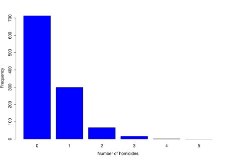

      

      Next, we propose a model for the data to begin addressing the question.

      It is proposed to model the data as iid (independent and identically distributed) draws from a Poisson distribution.

      Why is this a suitable model?

      What assumptions are being made?

      Are these assumptions reasonable?

      The probability mass function (pmf) for the poisson distribution is given by

      $$\mathrm{Pr}[X=x]=\frac{{\lambda }^x\exp (-\lambda )}{x!},$$

      for $x=0,1,2,\mathrm{\dots }$, so it still remains to make a sensible choice for the parameter $\lambda$. As before, we will make an estimate of $\lambda$ based on our data; the equation we use to produce the estimate will be a different estimator than in Part 1.

      12.2 What is likelihood?

      In the last example we discussed that a model for observed data typically has unknown parameters that we need to estimate. We proposed to model the London homicide data by a Poisson distribution. How do we estimate the parameter? In Math104 you met the method of moments estimator (MOME); whilst it is often easy to compute, the estimators it yields can often be improved upon; for this reason it has mostly been superceded by the method of maximum likelihood.

      Definition.

      Suppose we have data $x_1,\mathrm{\dots },x_n$, that arise from a population with pmf (or pdf) $f(\cdot )$, with at least one unknown parameter $\theta$. Then the likelihood function of the parameter $\theta$ is the probability (or density) of the observed data for given values of $\theta$.

      If the data are iid, the likelihood function is defined as

      $$L(\theta |x_1,\mathrm{\dots },x_n)=\prod _{i=1}^{n}f(x_i|\theta ).$$

      The product arises because we assume independence, and joint probabilities (or densities) obey a product law under independence (Math230).

      TheoremExample 12.2.1 London homicides continued

      For the Poisson example, recall that the probability mass function (pmf) for the Poisson distribution is given by

      $$\mathrm{Pr}[X=x]=\frac{{\lambda }^x\exp (-\lambda )}{x!}.$$

      We will always keep things general to begin by talking in terms of data $x_1,\mathrm{\dots },x_n$, rather than the actual data from the table. From the above definition, the likelihood function of the unknown parameter $\lambda$ is

      $$L(\lambda |x_1,\mathrm{\dots },x_n)=\prod _{i=1}^n\frac{{\lambda }^{x_i}\exp (-\lambda )}{x_i!}.$$

      Let’s have a look at how the likelihood function behaves for different values of $\lambda$. To keep things simple, let’s take just a random sample of 20 days.

      ⬇

      set.seed(1)

      #read in the data

      x<-c(rep(0,713),rep(1,299),rep(2,66),rep(3,16),4)

      %\end{lstlisting}

      \begin{lstlisting}

      #take a sample: 20 observations

      xs<-sample(x,20)

      ⬇

      #likelihood function

      L<-function(lam){

      m<-length(lam)

      sapply(1:m, function(i) prod(dpois(xs,lam[i])))

      }

      ⬇

      #values of lambda to plot (trial and error..)

      lam<-seq(from=0.3,to=1.1,length=100)

      plot(lam,L(lam),type="l")

      

      What does the likelihood plot tell us?

      Definition.

      Maximum likelihood estimator/estimate. For given data $x_1,\mathrm{\dots },x_n$, the maximum likelihood estimate (MLE) of $\theta$ is the value of $\theta$ that maximises $L(\theta |x_1,\mathrm{\dots },x_n)$, and is denoted $\widehat{\theta }$. The maximum likelihood estimator of $\theta$ based on random variables $X_1,\mathrm{\dots },X_n$ will be denoted $\widehat{\theta }(𝐗)$.

      So the MLE, $\widehat{\theta }$, is the value of $\theta$ where the likelihood is the largest. This is intuitively sensible.

      It is often computationally more convenient to take logs of the likelihood function.

      Definition.

      The log-likelihood function is the natural logarithm of the likelihood function and, for iid data $x_1,\mathrm{\dots },x_n$ is denoted thus:

      	$l(\theta |x_1,\mathrm{\dots },x_n)=\log \{L(\theta |x_1,\mathrm{\dots },x_n)\}$	$=\log \left\{{\displaystyle \prod _{i=1}^n}f(x_i|\theta )\right\}$
      		$={\displaystyle \sum _{i=1}^n}\log \left\{f(x_i|\theta )\right\}.$

      One reason that this is a good thing to do is it means we can switch the product to a sum, which is easier to deal with algebraically.

      IMPORTANT FACT: Since ‘log’ is a monotone increasing function, $\widehat{\theta }$ maximises the log-likelihood if and only if it maximises the likelihood; if we want to find an MLE we can choose which of these functions to try and maximise.

      Let us return to the Poisson model. The log-likelihood function for the Poisson data is

      	$l(\lambda |𝐱)$	$={\displaystyle \sum _{i=1}^n}\log \left\{{\displaystyle \frac{{\lambda }^{x_i}\exp (-\lambda )}{x_i!}}\right\}$
      		$={\displaystyle \sum _{i=1}^n}\left\{\log ({\lambda }^{x_i})+\log (\exp (-\lambda ))-\log (x_i!)\right\}$
      		$={\displaystyle \sum _{i=1}^n}\left\{x_i\log (\lambda )-\lambda -\log (x_i!)\right\}$
      		$=\log (\lambda ){\displaystyle \sum _{i=1}^n}{x}_i-n\lambda -{\displaystyle \sum _{i=1}^n}\log (x_i!).$

      We can now use the maximisation procedure of our choice to find the MLE. A sensible approach in this case is differentiation.

      $$\frac{\partial }{\partial \lambda }l(\lambda |𝐱)=\frac{1}{\lambda }\sum _{i=1}^n{x}_i-n.$$

      Now if we solve $\frac{\partial }{\partial \lambda }l(\lambda |𝐱)=0$, this gives us potential candidate(s) for the MLE. For the above, there is only one solution:

      ${\widehat{\lambda }}^{-1}{\displaystyle \sum _{i=1}^n}{x}_i-n=0$

      i.e.

      $\widehat{\lambda }={\displaystyle \frac{{\sum }_{i=1}^n{x}_i}{n}}=\overline{x}.$

      To confirm that this really is the MLE, we need to verify it is a maximum:

      It is clear intuitively that this is a sensible estimator; let’s formalise that into two desirable features we may look for in a ‘good’ estimator. We recall these properties (which you have met before):

      Now plugging in the value of $\overline{x}$ we find that

      $$\widehat{\lambda }=\frac{(0\times 713)+(1\times 299)+(2\times 66)+(3\times 16)+(4\times 1)}{713+299+66+16+1}=\frac{483}{1095}.$$

      Plugging in the actual numerical values of the data at the last minute is good practice, as it means we have solved a more general problem, and helps us to remember about sampling variation.

      The next step is to check that the Poisson model gives a reasonable fit to the data.

      Plotting the observed data against the expected data under the assumed model is a useful technique here.

      ⬇

      > #value of lambda from mom

      > momlam<-483/1095

      > #expected data counts

      > expdata<-1095*dpois(0:5,momlam)

      > #make plot

      > barplot(rbind(obsdata,expdata),names.arg=0:5,xlab=

      "Number of homicides",ylab="Frequency"

      col=c("blue","green"),beside=T)

      > #add legend

      > legend("topright",c("observed","expected"),

      col=c("blue","green"),lty=1)

      

      The fit looks very good!

      Let us now compare this to another estimator you already know: the method of moments estimator from Math104.

      Definition.

      Let $X_1,\mathrm{\dots },X_n$ be an iid sample from pmf or pdf $f(\cdot |\theta )$, where $\theta$ is one-dimensional. Then the method of moments estimator (MOME) $\widehat{\theta }$ solves

      $${𝔼}_{\widehat{\theta }}[X]=\frac{1}{n}\sum _{i=1}^n{X}_i.$$

      The left hand side is the theoretical moment and the right hand side is the sample moment. What this means is that we should choose the value of $\widehat{\theta }$ such that the sample mean is equal to the theoretical mean.

      In our example, recall that for a Poisson distributed random variable, $𝔼[X]=\lambda$. Therefore the MOME for $\lambda$ is

      $$\widehat{\lambda }=\frac{1}{n}\sum _{i=1}^n{X}_i.$$

      Notice that the MLE coincides with the MOME. We should be glad it does in this case, because the estimator is clearly sensible!

      Whenever the MOME and MLE disagree, the MLE is to be preferred. Much of the rest of this part of the course sets out why that is the case.

      Finally, we need to provide an answer to the original question.

      Four homicides were observed in London on 10 July 2008. Is this figure a cause for concern?

      The probability, on a given day, of seeing four or more homicides under the assumed model, where $X\sim \mathrm{Poisson}(\widehat{\lambda }=\frac{483}{1095})$, is given by

      by Math230 or R.

      But what must be borne in mind is that we can say this about any day of the year.

      Assuming days are independent (which we did anyway when fitting the Poisson distribution earlier), if $Y$ is the number of times we see 4 or more homicides in a year, then $Y\sim \mathrm{Binomial}(365,0.0011)$, and

      $\mathrm{Pr}[Y\ge 1]=1-\mathrm{Pr}[Y=0]=0.33.$

      So there is a chance of approximately $1/3$ that we see 4 or more homicides on at least one day in a given year.

      Some R code for the above:

      ⬇

      > #P[X>=4]:

      > ans1<-1-ppois(3,momlam)

      > #P[Y>=1]:

      > ans2<-1-dbinom(0,365,ans1)

      12.3 Likelihood Examples: continuous parameters

      We now explore examples of likelihood inference for some common models.

      TheoremExample 12.3.1 Accident and Emergency

      Accident and emergency departments are hard to manage because patients arrive at random (they are unscheduled). Some patients may need to be seen urgently.

      

      Excess staff (doctors and nurses) must be avoided because this wastes NHS money; however, A&E departments also have to adhere to performance targets (e.g. patients dealt with within four hours). So staff levels need to be ‘balanced’ so that there are sufficient staff to meet targets but not too many so that money is not wasted.

      A first step in achieving this is to study data on patient arrival times. It is proposed that we model the time between patient arrivals as iid realisations from an Exponential distribution.

      Why is this a suitable model?

      What assumptions are being made?

      Are these assumptions reasonable?

      Suppose I stand outside Lancaster Royal Infirmary A&E and record the following inter-arrival times of patients (in minutes):

      18.39, 2.70, 5.42, 0.99, 5.42, 31.97, 2.96, 5.28, 8.51, 10.90.

      As usual, the first thing we do is look at the data!

      ⬇

      arrive<-c(18.39,2.70,5.42,0.99,5.42,31.97,2.96,5.28,8.51,10.90)

      stripchart(arrive,pch=4,xlab="inter-arrival time (mins)")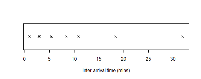

      

      The exponential pdf is given by

      $$f(x)=\lambda \exp (-\lambda x),$$

      for $x\ge 0$, $\lambda \ge 0$. Assuming that the data are iid, the definition of the likelihood function for $\lambda$ gives us, for general data $x_1,\mathrm{\dots },x_n$,

      $$L(\lambda )=\prod _{i=1}^n\lambda \exp (-\lambda x_i).$$

      Note: we usually drop the ‘$\mathrm{|}\mathrm{x}$’ from $L\mathrm{(}\lambda \mathrm{|}\mathrm{x}\mathrm{)}$ whenever possible.

      Usually, when we have products and the parameter is continuous, the best way to find the MLE is to find the log-likelihood and differentiate.

      So the log-likelihood is

      	$l(\lambda )$	$={\displaystyle \sum _{i=1}^n}\log \left\{\lambda \exp (-\lambda x_i)\right\}$
      		$={\displaystyle \sum _{i=1}^n}\left\{\log (\lambda )-\lambda x_i\right\}$
      		$=n\log (\lambda )-\lambda {\displaystyle \sum _{i=1}^n}{x}_i.$

      Now we differentiate:

      $$\frac{\partial }{\partial \lambda }l(\lambda )=l^{\prime }(\lambda )=\frac{n}{\lambda }-\sum _{i=1}^n{x}_i.$$

      Now solutions to $l^{\prime }(\lambda )=0$ are potential MLEs.

      1. 1

         $\frac{n}{\widehat{\lambda }}-{\sum }_{i=1}^n{x}_i=0,$

      2. 2

         $\widehat{\lambda }=\frac{n}{{\sum }_{i=1}^n{x}_i}=\frac{1}{\overline{x}}.$

      To ensure this is a maximum we check the second derivative is negative:

      So the solution we have found is the MLE, and plugging in our data we find (via 1/mean(arrive))

      $$\widehat{\lambda }=0.108.$$

      Now that we have our MLE, we should check that the assumed model seems reasonable. Here, we will use a QQ-plot.

      ⬇

      #MLE of lambda (rate)

      lam<-1/mean(arrive)

      #1/(n+1), 2/(n+1),..., n/(n+1).

      quant<-seq(from=1/11,to=10/11,length=10)

      #produce QQ-plot

      qqplot(qexp(quant,rate=lam),arrive,xlab="Theoretical

      quantiles",ylab="Actual")

      #add line of equality

      abline(0,1)

      

      Given the small dataset, this seems ok – there is no obvious evidence of deviation from the exponential model.

      Knowing that the exponential distribution is reasonable, and having an estimate for its rate, is useful to calculate staff scheduling requirements in the A&E.

      Extensions of the idea consider flows of patients through the various services (take Math332 Stochastic Processes and/or the STOR-i MRes for more on this).

      TheoremExample 12.3.2 Is human body temperature really 98.6 degrees Fahrenheit?

      In an article by Mackowiak et al.³³Mackowiak P.A., Wasserman, S.S. and Levine, M.M. (1992) A Critical Appraisal of 98.6 Degrees F, the Upper Limit of the Normal Body Temperature and Other Legacies of Carl Reinhold August Wunderlich, the authors measure the body temperatures of a number of individuals to assess whether true mean body temperature is 98.6 degrees Fahrenheit or not. A dataset of $130$ individuals is available in the normtemp dataset. The data are assumed to be normally distributed with standard deviation $0.73$.

      Why is this a suitable model?

      What assumptions are being made?

      Are these assumptions reasonable?

      What do the data look like?

      

      The plot can be produced using

      ⬇

      > load("normtemp.Rdata")

      > hist(normtemp$temperature)

      The histogram of the data is reasonable, but there might be some skew in the data (right tail).

      The normal pdf is given by

      $$f(x|\mu ,\sigma )=\frac{1}{\sqrt{2\pi {\sigma }^2}}\exp \{-\frac{{(x_i-\mu )}^2}{2{\sigma }^2}\},$$

      where in this case, $\sigma$ is known.

      The likelihood is then

      	$L(\mu |x_1,\mathrm{\dots },x_n)$	$={\displaystyle \prod _{i=1}^n}{\displaystyle \frac{1}{\sqrt{2\pi {\sigma }^2}}}\exp \left\{-{\displaystyle \frac{{(x_i-\mu )}^2}{2{\sigma }^2}}\right\}$
      		$={\left(2\pi {\sigma }^2\right)}^{-n/2}\exp \left\{-{\displaystyle \sum _{i=1}^n}{\displaystyle \frac{{(x_i-\mu )}^2}{2{\sigma }^2}}\right\}.$

      Since the parameter of interest (in this case $\mu$) is continuous, we can differentiate the log-likelihood to find the MLE:

      $$l(\mu )=-\frac{n}{2}\log (2\pi {\sigma }^2)-\frac{1}{2{\sigma }^2}\sum _{i=1}^n{(x_i-\mu )}^2$$

      and so

      $$l^{\prime }(\mu )=-\frac{1}{2{\sigma }^2}\sum _{i=1}^n(-2)(x_i-\mu ).$$

      For candidate MLEs we set this to zero and solve, i.e.

      	${\displaystyle \frac{1}{{\sigma }^2}}{\displaystyle \sum _{i=1}^n}{x}_i-n\widehat{\mu }$	$=0$
      	${\displaystyle \sum _{i=1}^n}{x}_i-n\widehat{\mu }$	$=0$

      and so the MLE is $\widehat{\mu }=\overline{x}$.

      This is also the “obvious” estimate (the sample mean). To check it is indeed an MLE, the second derivative of the log-likelihood is

      which confirms this is the case.

      Using the data, we find $\widehat{\mu }=\overline{x}=98.25$.

      This might indicate evidence for the body temperature being different from the assumed 98.6 degrees Fahrenheit.

      We now check the fit:

      ⬇

      > temps <-normtemp$temperature   # for shorthand

      > mean(temps)

      [1] 98.24923

      > stdtemp = (temps - mean(temps))/0.73

      > qqnorm(stdtemp)

      > abline(0,1)   # add "ideal" fit line y = x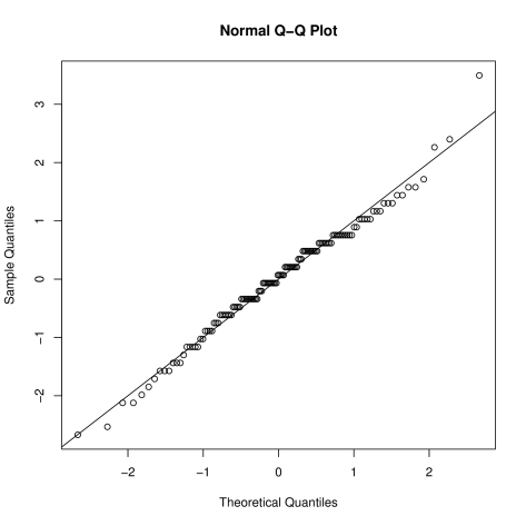

      

      The fit looks good – although (as the histogram previously showed) there is possibly some mild right (positive) skew, indicated by the quantile points above the $y=x$ line.

      Why might the QQ-plot show the “stepped” behaviour of the points?

      

      TheoremExample 12.3.3

      Every day I cycle to Lancaster University, and have to pass through the traffic lights at the crossroads by Booths (heading south down Scotforth Road). I am either stopped or not stopped by the traffic lights. Over a period of a term, I cycle in 50 times. Suppose that the time I arrive at the traffic lights is independent of the traffic light sequence.

      On 36 of the 50 days, the lights are on green and I can cycle straight through. Let $\theta$ be the probability that the lights are on green. Write down the likelihood and log-likelihood of $\theta$, and hence calculate its MLE.

      With the usual iid assumption we see that, if $R$ is the number of times the lights are on green then $R\sim \text{Binomial}(50,\theta )$. So we have

      $$\mathrm{Pr}[R=36]=\left(\genfrac{}{}{0pt}{}{50}{36}\right){\theta }^{36}{(1-\theta )}^{14}.$$

      We therefore have, for general $r$ and $n$,

      $$L(\theta )=\left(\genfrac{}{}{0pt}{}{n}{r}\right){\theta }^r{(1-\theta )}^{n-r},$$

      and

      $$l(\theta )=K+r\log (\theta )+(n-r)\log (1-\theta ).$$

      Solutions to $l^{\prime }(\theta )=0$ are potential MLEs:

      $$l^{\prime }(\theta )=\frac{r}{\theta }-\frac{n-r}{1-\theta },$$

      and if $l^{\prime }(\widehat{\theta })=0$ we have

      	${\displaystyle \frac{r}{\widehat{\theta }}}=$	$\mathrm{ }{\displaystyle \frac{n-r}{1-\widehat{\theta }}}$
      	$\text{i.e.}\mathit{\hspace{1em}\hspace{1em}}\widehat{\theta }=$	$\mathrm{ }{\displaystyle \frac{\stackrel{}{r}}{n}}.$

      For this to be an MLE it must have negative second derivative.

      In particular we have $r=36$ and $n=50$ so $\widehat{\theta }=36/50$ is the MLE.

      Now suppose that over a two week period, on the 14 occasions I get stopped by the traffic lights (they are on red) my waiting times are given by (in seconds)

      $$4.2,6.9,13.7,2.8,19.3,10.4,1.0,19.4,18.6,0.6,4.5,12.9,0.5,16.0.$$

      Assume that the traffic lights remain on red for a fixed amount of time $t_r$, regardless of the traffic conditions.

      Given the above data, write down the likelihood of $t_r$, and sketch it. What is the MLE of $t_r$?

      We are going to assume that these waiting times are drawn independently from $\mathrm{Uniform}[0,t_r]$, where $t_r$ is the parameter we wish to estimate.

      Why is this a suitable model?

      What assumptions are being made?

      Are these assumptions reasonable?

      Constructing the likelihood for this example is slightly different from those we have seen before. The pdf of the $\mathrm{Uniform}(0,t_r)$ distribution is

      The unusual thing here is that the data enters only through the boundary conditions on the pdf. Another way to write the above pdf is

      $$f(x)=t_r^{-1}\mathrm{𝟏}[0\le x\le t_r],$$

      where $\mathrm{𝟏}$ is the indicator function.

      For data $x_1,\mathrm{\dots },x_n$, the likelihood function is then

      $$L(t_r)=\prod _{i=1}^n{t}_r^{-1}\mathrm{𝟏}[0\le x_i\le t_r].$$

      We can write this as

      	$L(t_r)$	$=t_r^{-n}\mathrm{𝟏}\left[\{0\le x_1\le t_r\}{\displaystyle \bigcap }\mathrm{\dots }{\displaystyle \bigcap }\{0\le x_n\le t_r\}\right]$
      		$=t_r^{-n}\mathrm{𝟏}[\max (x_i)\le t_r].$

      For our case we have $n=14$ and $\max (x_i)=19.4$, so $L(t_r)=t_r^{-14}\mathrm{𝟏}[19.4\le t_r]$ .

      We are next asked to sketch this MLE. In R,

      ⬇

      > maxx<-19.4

      > #values of t_r to plot

      > t<-seq(from=18,to=22,length=1000)

      >

      > #likelihood function

      > uniflik<-function(t){

      > t^(-14)*(t>=19.4)

      > }

      >

      > plot(t,uniflik(t),type="l")

      

      From the plot it is clear that ${\widehat{t}}_r=19.4=\max (x_i)$, since this is the value that leads to the maximum likelihood. Notice that solving $l^{\mathrm{\prime }}\mathit{}\mathrm{(}{t}_r\mathrm{)}\mathrm{=}\mathrm{0}$ would not work in this case, since the likelihood is not differentiable at the MLE.

      However, on the feasible range of $t_r$, i.e. $\max (x_i)\le t_r$, we have

      $$l(t_r)=-n\log (t_r),$$

      and so

      $$l^{\prime }(t_r)=-n/t_r.$$

      Remember that derivatives express the rate of change of a function. Hence since the (log-)likelihood is negative ($t_r>0$ is strictly positive), then the likelihood is decreasing on the feasible range of parameter values.

      Since we are trying to maximise the likelihood, this means we should take the minimum over the feasible range as the MLE. The minimum value on the range $\max (x_i)\le t_r$ is ${\widehat{t}}_r=\max (x_i)=19.4$.

      12.4 Likelihood Examples: discrete parameters

      One case where differentiation is clearly not the right approach to use for maximisation is when the parameter of interest is discrete.

      TheoremExample 12.4.1 Illegal downloads

      A computer network comprises of $m$ computers. The probability of one of these computers to store illegally downloaded files is $0.3$, independent for each computer. In a particular network it is found that exactly one computer contains illegally downloaded files. Our parameter of interest is $m$.

      What is a suitable model for the data?

      What assumptions are being made?

      Are these assumptions reasonable?

      What is the likelihood of $m$?

      Let $X\sim Bin(m,0.3)$ be the number of computers in the network that contains illegally downloaded files. Then $\mathrm{Pr}(\text{obs}|m)$ is

      $$L(m)=\mathrm{Pr}(X=1|m)=\left(\genfrac{}{}{0pt}{}{m}{1}\right){0.3}^1\times {0.7}^{m-1}=\frac{0.3}{0.7}{0.7}^{m}m.$$

      Note that the possible values $m$ can take are $m=1,2,\mathrm{\dots }$. We can sketch the likelihood for a suitable range of values:

      ⬇

      > mrange<-0:20 # value for m=0 will be zero

      > plot(mrange,dbinom(1,mrange,0.3),xlab="m",ylab="L(m)")

      

      From the plot, we can see that the MLE for $m$ is $\widehat{m}=3$. Alternatively, from the likelihood we have

      $$\frac{L(m+1)}{L(m)}=\frac{{0.3}^1\times {0.7}^m(m+1)}{{0.3}^1\times {0.7}^{m-1}m}=\frac{0.7(m+1)}{m}.$$

      The likelihood is increasing for $L(m+1)>L(m)$, which is equivalent to .

      To maximize the likelihood, we want the largest (integer) value of $m$ satisfying this constraint, i.e. $m=2$, hence $\widehat{m}=3$.

      Relative Likelihood intervals

      The ratio between two likelihood values is useful to look at for other reasons.

      Definition.

      Suppose we have data $x_1,\mathrm{\dots },x_n$, that arise from a population with likelihood function $L(\theta )$, with MLE $\widehat{\theta }$. Then the relative likelihood of the parameter $\theta$ is

      $$R(\theta )=\frac{L(\theta |𝐱)}{L(\widehat{\theta }|𝐱)}.$$

      The relative likelihood quantifies how likely different values of $\theta$ are relative to the maximum likelihood estimate.

      Using this definition, we can construct relative likelihood intervals which are similar to confidence intervals.

      Definition.

      A p% relative likelihood interval for $\theta$ is defined as the set

      $$\left\{\theta \right|R(\theta )\ge \frac{p}{100}\}.$$

      TheoremExample 12.4.2 Illegal downloads (cont.)

      For example a 50% relative likelihood interval for $m$ in our example would be

      	$\left\{m\right|R(m)\ge 0.5\}$	$=\left\{m\right|{\displaystyle \frac{{0.3}^1\times {0.7}^{m-1}m}{{0.3}^1\times {0.7}^2\times 3}}\ge 0.5\}$
      		$=\left\{m\right|{0.7}^{m-3}m\ge 1.5\}$

      By plugging in different values of $m$, we see that the relative likelihood interval is $\{1,\mathrm{\dots },7\}$. The values in the interval can be seen in the figure below.

      

      TheoremExample 12.4.3 Sequential sampling with replacement: Smarties colours

      Suppose we are interested in estimating $m$, the number of distinct colours of Smarties.

      

      In order to estimate $m$, suppose members of the class make a number of draws and record the colour.

      Suppose that the data collected (seven draws) were:

      purple, blue, brown, blue, brown, purple, brown.

      We record whether we had a new colour or repeat:

      New, New, New, Repeat, Repeat, Repeat, Repeat.

      Let $m$ denote the number of unique colours. Then the likelihood function for $m$ given the above data is:

      $$L(m|{𝐱}_{\mathrm{𝟏}})=1\times \frac{m-1}{m}\times \frac{m-2}{m}\times \frac{3}{m}\times \frac{3}{m}\times \frac{3}{m}\times \frac{3}{m}.$$

      If in a second experiment, we observed:

      New, New, New, Repeat, New, Repeat, New,

      then the likelihood would be:

      $$L(m|{𝐱}_{\mathrm{𝟐}})=1\times \frac{m-1}{m}\times \frac{m-2}{m}\times \frac{3}{m}\times \frac{m-3}{m}\times \frac{4}{m}\times \frac{m-4}{m}.$$

      The MLEs in each case are $\widehat{m}=3$ and $\widehat{m}=8$.

      The plots below show the respective likelihoods.

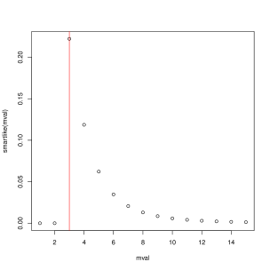
      R code for plotting these likelihoods:

      ⬇

      > # experiment 1:

      > smartlike<-function(m){

      > L<-1*(m-1)*(m-2)*(3)*(3)*(3)*(3)/m^6

      > }

      > mval<-1:15

      > plot(mval,smartlike(mval))

      > abline(v=3,col=2)

      > which.max(smartlike(mval))

      ⬇

      > # Experiment 2:

      > # e.g. pink, purple, blue, blue, brown, purple, orange

      > smartlike2<-function(m){

      > L<-1*(m-1)*(m-2)*(3)*(m-3)*(4)*(m-4)/m^6

      > }

      > dev.new()

      > plot(mval,smartlike2(mval))

      > abline(v=8,col=2)

      > which.max(smartlike2(mval))

      TheoremExample 12.4.4 Brexit opinions

      Three randomly selected members of a class of 10 students are canvassed for their opinion on Brexit. Two are in favour of staying in Europe. What can one infer about the overall class opinion?

      The parameter in this model is the number of pro-Remain students in the class, $m$, say. It is discrete, and could take values $0,1,2,\mathrm{\dots },10$. The actual true unknown value of $m$ is designated by $m_{\text{true}}$.

      Now $\mathrm{Pr}(\text{obs}|m)$ is

      $\mathrm{Pr}(\text{2 in favour from }m\text{ and 1 against from }10-m).$

      Now since the likelihood function of $m$ is the probability (or density) of the observed data for given values of $m$, we have

      	$L(m)$	$={\displaystyle \frac{\left(\genfrac{}{}{0pt}{}{m}{2}\right)\left(\genfrac{}{}{0pt}{}{10-m}{1}\right)}{\left(\genfrac{}{}{0pt}{}{10}{3}\right)}}$
      		$={\displaystyle \frac{m(m-1)(10-m)}{240}}$

      for $m=2,3,\mathrm{\dots },9$.

      This function is not continuous (because the parameter $m$ is discrete). It can be maximised but not by differentiation.

      

      ⬇

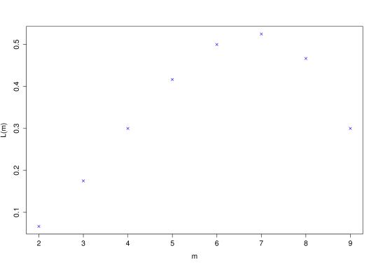      > #likelihood function

      > L<-function(m){

      > choose(m,2)*choose(10-m,1)/choose(10,3)

      > }

      > #values of m to plot

      > m<-2:9

      > plot(m,L(m),pch=4,col="blue")

      The maximum likelihood estimate is $\widehat{m}=7.$ Note that the points are not joined up in this plot. This is to emphasize the discrete nature of the parameter of interest.

      The probability model is an instance of the hypergeometric distribution.

      12.5 Summary

      {mdframed}

      A procedure for modelling and inference:

      1. 1

         Subject-matter question needs answering.

      2. 2

         Data are, or become, available to address this question.

      3. 3

         Look at the data – exploratory analysis.

      4. 4

         Propose a model.

      5. 5

         Check the model fits.

      6. 6

         Use the model to address the question.

      • 1

        The likelihood function is the probability of the observed data for instances of a parameter. Often we use the log-likelihood function as it is easier to work with. The likelihood is a function of an unknown parameter.

      • 2

        The maximum likelihood estimator (MLE) is the value of the parameter that maximises the likelihood. This is intuitively appealing, and later we will show it is a theoretically justified choice. The MLE should be found using an appropriate maximisation technique.

      • 3

        If the parameter is continuous, we can often (but not always) find the MLE by considering the derivative of the log-likelihood. If the parameter is discrete, we usually evaluate the likelihood at a range of possible values.

        DON’T JOIN UP POINTS WHEN PLOTTING THE LIKELIHOOD FOR A DISCRETE PARAMETER.

        DO NOT DIFFERENTIATE LIKELIHOODS OF DISCRETE PARAMETERS!

      Chapter 13 Information and Sufficiency

      13.1 Introduction

      Last time we looked at some more examples of the method of maximum likelihood. When the parameter of interest, $\theta$, is continuous, the MLE, $\widehat{\theta }$, can be found by differentiating the log-likelihood and setting it equal to zero. We must then check the second derivative of the log-likelihood is negative (at our candidate $\widehat{\theta }$) to verify that we have found a maximum.

      Definition.

      Suppose we have a sample $𝐱=x_1,\mathrm{\dots },x_n$, drawn from a density $f(𝐱|\theta )$ with unknown parameter $\theta$, with log-likelihood $l(\theta |𝐱)$. The score function, $S(\theta )$, is the first derivative of the log-likelihood with respect to $\theta$:

      $$S(\theta |𝐱)=l^{\prime }(\theta |𝐱)=\frac{\partial }{\partial \theta }l(\theta |𝐱).$$

      This is just giving a name to something we have already encountered.

      As discussed previously, the MLE solves $S(\widehat{\theta })=0$. Here, $f(𝐱|\theta )$ is being used to denote the joint density of $𝐱=x_1,\mathrm{\dots },x_n$. For the iid case, $f(𝐱|\theta )={\prod }_{i=1}^{n}f(x_i|\theta )$. Also, $l(\theta |𝐱)=\log f(𝐱|\theta )$. This is all just from the definitions.

      Definition.

      Suppose we have a sample $𝐱=x_1,\mathrm{\dots },x_n$, drawn from a density $f(𝐱|\theta )$ with unknown parameter $\theta$, with log-likelihood $l(\theta |𝐱)$. The observed information function, $I_O(\theta )$, is MINUS the second derivative of the log-likelihood with respect to $\theta$:

      $$I_O(\theta |𝐱)=-l^{\prime \prime }(\theta |𝐱)=-\frac{{\partial }^2}{\partial {\theta }^2}l(\theta |𝐱).$$

      Remember that the second derivative of $l(\theta )$ is negative at the MLE $\widehat{\theta }$ (that’s how we check it’s a maximum!). So the definition of observed information takes the negative of this to give something positive.

      The observed information gets its name because it quantifies the amount of information obtained from a sample. An approximate 95% confidence interval for ${\theta }_{\text{true}}$ (the unobservable true value of the parameter $\theta$) is given by

      $$(\widehat{\theta }-\frac{1.96}{\sqrt{I_O(\widehat{\theta })}},\widehat{\theta }+\frac{1.96}{\sqrt{I_O(\widehat{\theta })}}).$$

      This confidence interval is asymptotic, which means it is accurate when the sample is large. Some further justification on where this interval comes from will follow later in the course.

      What happens to the confidence interval as $I_O(\widehat{\theta })$ changes?

      TheoremExample 13.1.1 Mercedes Benz drivers

      You may recall the following example from last year.The website MBClub UK (associated with Mercedes Benz) carried out a poll on the number of times taken to pass a driving test. The results were as follows.

      Number of failed attempts	0	1	2	$\ge 3$
      Observed frequency	147	47	20	5

      As always, we begin by looking at the data.

      

      ⬇

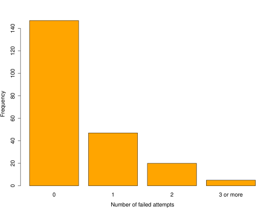      obsdata<-c(147,47,20,5)

      barplot(obsdata,names.arg=c(0:2, or more'),

      xlab="Number of failed attempts",

      ylab="Frequency",col="orange")

      Next, we propose a model for the data to begin addressing the question.

      It is proposed to model the data as iid (independent and identically distributed) draws from a geometric distribution.

      Why is this a suitable model?

      What assumptions are being made?

      Are these assumptions reasonable?

      The probability mass function (pmf) for the geometric distribution, where $X$ is defined as the number of failed attempts, is given by

      $$\mathrm{Pr}[X=x]=\theta {(1-\theta )}^x,$$

      where $x=0,1,2,\mathrm{\dots }$.

      Assuming that the people in the ‘3 or more’ column failed exactly three times, the likelihood for general data $x_1,\mathrm{\dots },x_n$ is

      $$L(\theta )=\prod _{i=1}^n\theta {(1-\theta )}^{x_i},$$

      and the log-likelihood is

      	$l(\theta )$	$={\displaystyle \sum _{i=1}^n}\log \left\{\theta {(1-\theta )}^{x_i}\right\}$
      		$={\displaystyle \sum _{i=1}^n}\{\log (\theta )+x_i\log (1-\theta )\}$
      		$=n\log (\theta )+\log (1-\theta ){\displaystyle \sum _{i=1}^n}{x}_i.$

      The score function is therefore

      $$S(\theta )=l^{\prime }(\theta )=\frac{n}{\theta }-\frac{{\sum }_{i=1}^n{x}_i}{1-\theta }.$$

      A candidate for the MLE, $\widehat{\theta }$, solves $S(\widehat{\theta })=0$:

      1. 1

         $\frac{n}{\widehat{\theta }}=\frac{{\sum }_{i=1}^n{x}_i}{1-\widehat{\theta }},$

      2. 2

         $n(1-\widehat{\theta })=\widehat{\theta }{\sum }_{i=1}^n{x}_i,$

      3. 3

         $n=\widehat{\theta }\left(n+{\sum }_{i=1}^n{x}_i\right),$

      4. 4

         $\widehat{\theta }=\frac{n}{n+{\sum }_{i=1}^n{x}_i}.$

      To confirm this really is an MLE we need to verify it is a maximum, i.e. a negative second derivative.

      In this case the function is clearly negative for all $\theta \in (0,1)$, if not we would just need to check this is the case at the proposed MLE.

      Now plugging in the numbers, $n=219$ and ${\sum }_{i=1}^n{x}_i=0\times 147+1\times 47+2\times 20+3\times 5=102$, we get

      $$\widehat{\theta }=\frac{219}{219+102}=0.682.$$

      This is the same answer as the ‘obvious one’ from intuition.

      But now we can calculate the observed information at $\widehat{\theta }$, and use this to construct a 95% confidence interval for ${\theta }_{\text{true}}$.

      	$I_O(\widehat{\theta })$	$=-l^{\prime \prime }(\widehat{\theta })$
      		$={\displaystyle \frac{n}{{\widehat{\theta }}^2}}+{\displaystyle \frac{{\sum }_{i=1}^n{x}_i}{{(1-\widehat{\theta })}^2}}$
      		$={\displaystyle \frac{219}{{0.682}^2}}+{\displaystyle \frac{102}{{(1-0.682)}^2}}$
      		$=1479.5.$

      Now the 95% confidence interval is given by

      	$(l,u)$	$=(\widehat{\theta }-{\displaystyle \frac{1.96}{\sqrt{I_O(\widehat{\theta })}}},\widehat{\theta }+{\displaystyle \frac{1.96}{\sqrt{I_O(\widehat{\theta })}}})$
      		$=(0.682-{\displaystyle \frac{1.96}{\sqrt{1479.5}}},0.682+{\displaystyle \frac{1.96}{\sqrt{1479.5}}})$
      		$=(0.631,0.733).$

      We should also check the fit of the model by plotting the observed data against the theoretical data from the model (with the MLE plugged in for $\theta$).

      ⬇

      #value of theta: MLE

      mletheta<-0.682

      #expected data counts

      expdata<-219*c(dgeom(0:2,mletheta),1-pgeom(2,mletheta))

      #make plot

      barplot(rbind(obsdata,expdata),names.arg=c(0:2, or more'),

      xlab="Number of failed attempts",ylab="Frequency",

      col=c("orange","red"),beside=T)

      #add legend

      legend("topright",c("observed","expected"),

      col=c("orange","red"),lty=1)

      

      We can do actually do slightly better than this.

      We assumed ‘the people in the “3 or more” column failed exactly three times’. With likelihood we don’t need to do this. Remember: the likelihood is just the joint probability of the data. In fact, people in the “3 or more” group have probability

      	$\mathrm{Pr}[X\ge 3]$	$=1-(\mathrm{Pr}[X=0]+\mathrm{Pr}[X=1]+\mathrm{Pr}[X=2])$
      		$=1-(\theta +(1-\theta )\theta +{(1-\theta )}^2\theta ).$

      We could therefore write the likelihood more correctly as

      $$L(\theta )=\prod _{i=1}^n{\left\{\theta {(1-\theta )}^{x_i}\right\}}^{z_i}\prod _{i=1}^n{\left\{1-(\theta +(1-\theta )\theta +{(1-\theta )}^2\theta )\right\}}^{1-z_i},$$

      where $z_i=1$ if and $z_i=0$ if $x_i\ge 3$.

      NOTE: if all we know about an observation $x$ is that it exceeds some value, we say that $x$ is censored. This is an important issue with patient data, as we may lose contact with a patient before we have finished observing them. Censoring is dealt with in more generality MATH335 Medical Statistics.

      What is the MLE of $\theta$ using the more correct version of the likelihood?

      The term in the second product (for the censored observations) can be seen as a geometric progression with constant term $a=\theta$ and common ratio $r=(1-\theta )$, and so $\mathrm{Pr}(X\ge 3|\theta )={(1-\theta )}^3$ (check that this is the case).

      Hence the likelihood can be written

      	$L(\theta )$	$={\theta }^{n_u}{(1-\theta )}^{\sum x_i}{\left({(1-\theta )}^3\right)}^{n_c}$
      		$={\theta }^{n_u}{(1-\theta )}^{\sum x_i+3n_c}$

      where the sum of $x_i$’s only involves the uncensored observations, $n_u$ denotes the number of uncensored observations, and $n_c$ is the number of censored observations.

      The log-likelihood becomes $l(\theta )=n_u\log (\theta )+(\sum x_i+3n_c)\log (1-\theta )$.

      Differentiating, the score function is

      $$S(\theta )=l^{\prime }(\theta )=\frac{n_u}{\theta }-\frac{\sum x_i+3n_c}{1-\theta }.$$

      A candidate MLE solves $l^{\prime }(\widehat{\theta })=0$, giving

      	${\displaystyle \frac{n_u}{\widehat{\theta }}}$	$={\displaystyle \frac{\sum x_i+3n_c}{1-\widehat{\theta }}}$
      	$n_u(1-\widehat{\theta })$	$=\widehat{\theta }\left({\displaystyle \sum x_i}+3n_c\right)$
      	$n_u$	$=\widehat{\theta }\left(n_u+{\displaystyle \sum x_i}+3n_c\right)$
      	$\widehat{\theta }$	$={\displaystyle \frac{n_u}{n_u+\sum x_i+3n_c}}.$

      The value of the MLE using these data is $\frac{214}{214+102}=0.677$.

      Compare this to the original MLE of 0.682.

      Why is the new estimate different to this?

      Why is the difference small?

      13.2 Suppression of Information

      Last time we introduced the score function (the derivative of the log-likelihood), and the observed information function (MINUS the second derivative of the log-likelihood). The score function is zero at the MLE. The observed information function evaluated at the MLE gives us a method to construct confidence intervals.

      We will now study the concept of observed information in more detail.

      

      TheoremExample 13.2.1 Human Genotyping

      Humans are a diploid species, which means you have two copies of every gene (one from your father, one from your mother). Genes occur in different forms; this is what leads to some of the different traits you see in humans (e.g. eye colour). Mendelian traits are a special kind of trait that are determined by a single gene.

      Having wet or dry earwax is a Mendelian trait. Earwax wetness is controlled by the gene ABCC11 (this gene lives about half way along chromosome 16). We will call the wet earwax version of ABCC11 W, and the dry version w. The wet version is dominant, which means you only need one copy of W to have wet earwax. Both copies of the gene need to be w to get dry earwax.

      The Hardy-Weinberg law of genetics states that if W occurs in a (randomly mating) population with proportion $p$ (so w occurs with proportion $(1-p)$) potential combinations in humans obey the proportions:

      combination	WW	Ww	ww
      proportion	$p^2$	$2p(1-p)$	${(1-p)}^2$

      Suppose I take a sample of 100 people and assess the wetness of their earwax. I observe that 87 of the people have wet earwax and 13 of them have dry earwax.

      I am actually interested in $p$, the proportion of copies of W in my population.

      Show that the probability of a person having wet earwax is $p(2-p)$, and that the probability of a person having dry earwax is ${(1-p)}^2$. Also show that these two probabilities sum to $1$.

      The number of people with wet earwax in my sample is therefore $\mathrm{Binomial}(100,p(2-p))$. So

      $$\mathrm{Pr}[\text{obs}|p]=\left(\genfrac{}{}{0pt}{}{100}{87}\right){\left\{p(2-p)\right\}}^{87}{\left\{{(1-p)}^2\right\}}^{13}.$$

      IMPORTANT FACT: when writing down the likelihood, we can always omit multiplicative constants, since they become additive in the log-likelihood, then disappear in the differentation. A multiplicative constant is one that does not depend on the parameter of interest (here $p$).

      So we can write down the likelihood as

      	$L(p)$	$\propto {\left\{p(2-p)\right\}}^{87}{\left\{{(1-p)}^2\right\}}^{13}$
      		$={\left\{p(2-p)\right\}}^{87}{(1-p)}^{26}.$

      So the log likelihood is

      	$l(p)$	$=87\log \left\{p(2-p)\right\}+26\log (1-p)$
      		$=87\log (p)+87\log (2-p)+26\log (1-p)$

      (plus constant).

      Now $p$ is a continuous parameter so a suitable way to find a candidate MLE is to differentiate. The score function is

      $$S(p)=l^{\prime }(p)=\frac{87}{p}-\frac{87}{2-p}-\frac{26}{1-p}.$$

      We can solve $S(\widehat{p})=0$; it is as a quadratic in $\widehat{p}$:

      1. 1

         $87(2-p)(1-p)-87p(1-p)-26p(2-p)=0,$

      2. 2

         $200{\widehat{p}}^2-400\widehat{p}+174=0,$

      3. 3

         $\frac{400\pm \sqrt{{400}^2-\mathrm{4.200.174}}}{2.200}=\widehat{p}.$

      This gives two solutions but we need $\widehat{p}\in [0,1]$ as it is a proportion, so get $\widehat{p}=0.639$ as our potential MLE.

      The second derivative is

      $$l^{\prime \prime }(p)=-\frac{87}{p^2}-\frac{87}{{(2-p)}^2}-\frac{26}{{(1-p)}^2}.$$

      This is clearly at $\widehat{p}$, confirming that it is a maximum.

      The observed information is obtained by substituting $\widehat{p}$ into $-l^{\prime \prime }(p)$, giving

      $$I_O(\widehat{p})=\frac{87}{{0.639}^2}+\frac{87}{{(2-0.639)}^2}+\frac{26}{{(1-0.639)}^2}=459.5.$$

      Hence an approximate 95% confidence interval for $p_{\text{true}}$ is given by

      	$(l,u)$	$=(\widehat{p}-{\displaystyle \frac{1.96}{\sqrt{I_O(\widehat{p})}}},\widehat{p}+{\displaystyle \frac{1.96}{\sqrt{I_O(\widehat{p})}}})$
      		$=(0.639-{\displaystyle \frac{1.96}{\sqrt{459.5}}},0.639+{\displaystyle \frac{1.96}{\sqrt{459.5}}})$
      		$=(0.548,0.730).$

      After all that derivation, don’t forget the context. This is a 95% confidence interval for the proportion of people with a W variant of ABCC11 gene in the population of interest.

      Suppose that, instead of looking in people’s ears to see whether their wax is wet or dry we decide to genotype them instead, thereby knowing whether they are WW, Ww or ww.

      This is a considerably more expensive option (although perhaps a little less disgusting) so a natural question is: what do we gain by doing this?

      We take the same 100 people and find that 42 are WW, 45 are Ww and 13 are ww. Think about how this relates back to the earwax wetness. Did we need to genotype everyone?

      The likelihood function for $p$ given our new information is

      	$L(p)\propto$	$\mathrm{ }{(p^2)}^{42}{\left\{2p(1-p)\right\}}^{45}{\left\{{(1-p)}^2\right\}}^{13}$
      		$=p^{84}{\left\{2p(1-p)\right\}}^{45}{(1-p)}^{26}.$

      The log-likelihood is

      	$l(p)$	$=84\log (p)+45\log \left\{2p(1-p)\right\}+26\log (1-p)$
      		$=84\log (p)+45\log (2)+45\log (p)+45\log (1-p)+26\log (1-p)$
      		$=129\log (p)+71\log (1-p)+c.$

      where $c$ is a constant.

      As before, $p$ is continuous so we can find candidates for the MLE by differentiating:

      $$S(p)=l^{\prime }(p)=\frac{129}{p}-\frac{71}{1-p}.$$

      Now solving $S(\widehat{p})=0$ gives a candidate MLE

      1. 1

         $\frac{129}{\widehat{p}}=\frac{71}{1-\widehat{p}}$,

      2. 2

         $129(1-\widehat{p})=71\widehat{p}$,

      i.e.

      $\widehat{p}={\displaystyle \frac{129}{200}}=0.645.$

      This is our potential MLE. Checking the second derivative

      $$l^{\prime \prime }(p)=-\frac{129}{p^2}-\frac{71}{{(1-p)}^2},$$

      which is at $\widehat{p}$ confirming that it is a maximum.

      The observed information is obtained by substituting $\widehat{p}$ into $-l^{\prime \prime }(p)$, giving

      $$I_O(\widehat{p})=\frac{129}{{0.645}^2}+\frac{71}{{(1-0.645)}^2}=873.5.$$

      Hence an approximate 95% confidence interval for $p_{\text{true}}$ is given by

      	$(l,u)$	$=(\widehat{p}-{\displaystyle \frac{1.96}{\sqrt{I_O(\widehat{p})}}},\widehat{p}+{\displaystyle \frac{1.96}{\sqrt{I_O(\widehat{p})}}})$
      		$=(0.645-{\displaystyle \frac{1.96}{\sqrt{873.5}}},0.645+{\displaystyle \frac{1.96}{\sqrt{873.5}}})$
      		$=(0.579,0.711).$

      Now, compare the confidence intervals and the observed informations from the two separate calculations. What do you conclude?

      Of course, genotyping the participants of the study is expensive, so may not be worthwhile. If this was a real problem, the statistician could communicate the figures above to the geneticist investigating gene ABCC11, who would then be able to make an evidence-based decision about how to conduct the experiment.

      13.3 Sufficiency

      Recall the driving test data from the Example 13.1.

      Number of failed attempts	0	1	2	$\ge 3$
      Observed frequency	147	47	20	5

      We chose to model these data as being geometrically distributed. Assuming that the people in the ‘3 or more’ column failed exactly three times, the log-likelihood for general data $x_1,\mathrm{\dots },x_n$ is

      	$l(\theta )$	$={\displaystyle \sum _{i=1}^n}\log \left\{\theta {(1-\theta )}^{x_i}\right\}$
      		$={\displaystyle \sum _{i=1}^n}\{\log (\theta )+x_i\log (1-\theta )\}$
      		$=n\log (\theta )+\log (1-\theta ){\displaystyle \sum _{i=1}^n}{x}_i.$

      Now, suppose that, rather than being presented with the table of passing attempts, you were simply told that with 219 people filling in the survey, ${\sum }_{i=1}^{219}{x}_i=102$.

      Would it still be possible to proceed with fitting the model?

      The answer is yes; moreover, we can proceed in exactly the same way, and achieve the same results! This is because, if you look at the log-likelihood, the only way in which the data is involved is through ${\sum }_{i=1}^n{x}_i$, meaning that in some sense, this is all we need to know.

      This is clearly a big advantage, we just have to remember one number rather than an entire table.

      We call ${\sum }_{i=1}^n{x}_i$ a sufficient statistic for $\theta$.

      Definition.

      Let $𝐱=x_1,\mathrm{\dots },x_n$ be a sample from $f(\cdot |\theta )$. Then a function of the data $T(𝐱)$ is said to be a sufficient statistic for $\theta$ (or sufficient for $\theta$) if $𝐱$ is independent of $\theta$ given $T(𝐱)$, i.e.

      $$\mathrm{Pr}[𝐗=𝐱|T(𝐱),\theta ]=\mathrm{Pr}[𝐗=𝐱|T(𝐱)].$$

      Some consequences of this definition:

      • 1

        For the objective of learning about $\theta$, if I am told $T(𝐱)$, there is no value in being told anything else about $𝐱$.

      • 2

        If I have two datasets ${𝐱}_{\mathrm{𝟏}}$ and ${𝐱}_{\mathrm{𝟐}}$, and $T({𝐱}_{\mathrm{𝟏}})=T({𝐱}_{\mathrm{𝟐}})$, then I should make the same conclusions about $\theta$ from both, even if ${𝐱}_{\mathrm{𝟏}}\ne {𝐱}_{\mathrm{𝟐}}$.

      • 3

        Sufficient statistics always exist since trivially $T(𝐱)=𝐱$ always satisfies the above definition.

      Definition.

      Let $𝐱=x_1,\mathrm{\dots },x_n$ be a sample from $f(\cdot |\theta )$. Let $T(𝐱)$ be sufficient for $\theta$. Then $T(𝐱)$ is said to be minimally sufficient for $\theta$ if there is no sufficient statistic with a lower dimension than $T$.

      Theorem (Neyman factorisation theorem).

      Let $\mathrm{x}\mathrm{=}{x}_{\mathrm{1}}\mathrm{,}\mathrm{\dots }\mathrm{,}{x}_n$ be a sample from $f\mathrm{(}\mathrm{\cdot }\mathrm{|}\theta \mathrm{)}$. Then a function $T\mathit{}\mathrm{(}\mathrm{x}\mathrm{)}$ is sufficient for $\theta$ if and only if the likelihood function can be factorised in the form

      $$L(\theta )=g(𝐱)\times h(T(𝐱),\theta ),$$

      where $g$ is a function of the data only, and $h$ is a function of the data only through $t\mathit{}\mathrm{(}\mathrm{x}\mathrm{)}$.

      For a proof see page 276 of Casella and Berger.

      We can also express the factorisation result in terms of the log-likelihood, which is often easier, just by taking logs of the above result:

      	$l(\theta )$	$=\log \left\{g(𝐱)\times h(T(𝐱),\theta )\right\}$
      		$=\log \{g(𝐱)\}+\log \{h(T(𝐱),\theta )\}$
      		$=\tilde{g}(𝐱)+\tilde{h}(T(𝐱),\theta ),$

      where $\tilde{g}=\log (g)$ and $\tilde{h}=\log (h)$.

      We can show that ${\sum }_{i=1}^n{x}_i$ is sufficient for $\theta$ in the driving test example by inspection of the log-likelihood:

      $$l(\theta )=n\log (\theta )+\log (1-\theta )\sum _{i=1}^n{x}_i.$$

      Letting $T(𝐱)={\sum }_{i=1}^n{x}_i$ , then $\tilde{h}(T(𝐱),\theta )=n\log (\theta )+\log (1-\theta )T(𝐱)$ , and $\tilde{g}(𝐱)=0$, we have satisfied the factorisation criterion, and hence $T(𝐱)={\sum }_{i=1}^n{x}_i$ is sufficient for $\theta$.

      Suppose that I carry out another survey on attempts to pass a driving test, again with $n=219$ participants and get data $\overrightarrow{y}=y_1,\mathrm{\dots },y_n$, with $𝐱\ne 𝐲$ but ${\sum }_{i=1}^n{x}_i={\sum }_{i=1}^n{y}_i$. Are the following statements true or false?

      1. 1

         $\widehat{\theta }(𝐱)$, the MLE based on data $𝐱$, is the same as $\widehat{\theta }(𝐲)$, the MLE based on data $𝐲$.

      2. 2

         The confidence intervals based on both datasets will be identical.

      3. 3

         The geometric distribution is appropriate for both datasets.

      An important shortcoming in only considering the sufficient statistic is that it does not allow us to check how well the chosen model fits.

      TheoremExample 13.3.1 Poisson parameter (cont.)

      Recall from the beginning of this section, the London homicides data, which we modelled as a random sample from the Poisson distribution. We found

      	$L(\lambda |x_1,\mathrm{\dots },x_n)$	$={\displaystyle \prod _{i=1}^n}{\displaystyle \frac{{\lambda }^{x_i}\exp (-\lambda )}{x_i!}}$
      		$={\lambda }^{{\sum }_i{x}_i}\exp (-n\lambda ){\displaystyle \prod _{i=1}^n}{\displaystyle \frac{1}{x_i!}}$
      		$\propto {\lambda }^{{\sum }_i{x}_i}\exp (-n\lambda ),$

      and that the log-likelihood function for the Poisson data is consequently

      $$l(\lambda )=\log (\lambda )\sum _{i=1}^n{x}_i-n\lambda +c,$$

      with the MLE being

      $$\widehat{\lambda }=\frac{{\sum }_{i=1}^n{x}_i}{n}=\overline{x}.$$

      By differentiating again, we can find the information function

      $$l^{\prime \prime }(\lambda |𝐱)=-{\lambda }^{-2}\sum _{i=1}^n{x}_i,$$

      and so

      $$I_O(\lambda |𝐱)={\lambda }^{-2}\sum _{i=1}^n{x}_i.$$

      What is a sufficient statistic for the Poisson parameter?

      For this case, we can let $T(𝐱)={\sum }_{i=1}^n{x}_i$, and $\tilde{h}(T(𝐱),\theta )=\log (\lambda )T(𝐱)-n\lambda$, and $\tilde{g}(𝐱)=c=-{\sum }_{i=1}^n\log (x_i!)$, we have satisfied the factorisation criterion, and hence $T(𝐱)={\sum }_{i=1}^n{x}_i$ is sufficient for $\lambda$.

      TheoremExample 13.3.2 Normal variance

      Suppose the sample $x_1,\mathrm{\dots },x_n$ comes from $X\sim N(0,\theta )$. Find a sufficient statistic for $\theta$. Is the MLE a function of this statistic or of the sample mean? Give a formula for the 95% confidence interval of $\theta$.

      First, the $\mathrm{Normal}(0,\theta )$ density is given by

      $f(x_i|\theta )={\displaystyle \frac{1}{\sqrt{2\pi \theta }}}\exp \{-{\displaystyle \frac{x_i^2}{2\theta }}\},$

      leading to the likelihood

      1. 1

         $L(\theta )={\prod }_{i=1}^n\frac{1}{\sqrt{2\pi \theta }}\exp \left\{-\frac{x_i^2}{2\theta }\right\},$

      2. 2

         $L(\theta )=\frac{1}{{\theta }^{n/2}}\exp \left\{-\frac{{\sum }_i{x}_i^2}{2\theta }\right\}.$

      Hence, $T(𝐱)={\sum }_i{x}_i^2$ is a sufficient statistic for $\theta$. The log-likelihood and score functions are

      1. 1

         $l(\theta )=-\frac{n}{2}\log \theta -\frac{{\sum }_i{x}_i^2}{2\theta },$

      2. 2

         $S(\theta )=l^{\prime }(\theta )=-\frac{n}{2\theta }+\frac{{\sum }_i{x}_i^2}{2{\theta }^2}.$

      Solving $S(\theta )=0$ gives a candidate MLE

      $\widehat{\theta }={\displaystyle \frac{{\sum }_i{x}_i^2}{n}},$

      which is a function of the sufficient statistic. To check this is an MLE we calculate

      $l^{\prime \prime }(\theta )={\displaystyle \frac{n}{2{\theta }^2}}-{\displaystyle \frac{{\sum }_i{x}_i^2}{{\theta }^3}}.$

      In this case it isn’t immediately obvious that , but substituting in

      	$l^{\prime \prime }(\widehat{\theta })$	$={\displaystyle \frac{n}{2{\left(\frac{\sum x_i^2}{n}\right)}^2}}-{\displaystyle \frac{\sum x_i^2}{{\left(\frac{\sum x_i^2}{n}\right)}^3}}$
      		$={\displaystyle \frac{n^3}{2{(\sum x_i^2)}^2}}-{\displaystyle \frac{n^3}{{(\sum x_i^2)}^2}}$

      confirming that this is an MLE.

      The observed information is $I_O(\widehat{\theta })=-l^{\prime \prime }(\widehat{\theta })$,

      $$I_O(\widehat{\theta })=\frac{n^3}{2{(\sum x_i^2)}^2}.$$

      Therefore a 95% confidence interval is given by

      	$(l,u)$	$=(\widehat{\theta }-{\displaystyle \frac{1.96}{\sqrt{I_O(\widehat{\theta })}}},\widehat{\theta }+{\displaystyle \frac{1.96}{\sqrt{I_O(\widehat{\theta })}}})$
      		$=({\displaystyle \frac{{\sum }_i{x}_i^2}{n}}-1.96n^{-3/2}{\displaystyle \sum x_i^2\sqrt{2}},{\displaystyle \frac{{\sum }_i{x}_i^2}{n}}+1.96n^{-3/2}{\displaystyle \sum x_i^2\sqrt{2}}).$

      13.4 Summary

      {mdframed}

      • 1

        The score function is the first derivative of the log-likelihood. The observed information is MINUS the second derivative of the log-likelihood. It will always be positive when evaluated at the MLE.

        DO NOT FORGET THE MINUS SIGN!

      • 2

        The likelihood function adjusts appropriately when more information becomes available. Observed information does what it says. Higher observed information leads to narrower confidence intervals. This is a good thing as narrower confidence intervals mean we are more sure about where the true value lies.

        For a continuous parameter of interest, $\theta$, the calculation of the MLE and its confidence interval follows the steps:

        1. 1

           Write down the likelihood, $L(\theta )$.

        2. 2

           Write down the log-likelihood, $l(\theta )$.

        3. 3

           Work out the score function, $S(\theta )=l^{\prime }(\theta )$.

        4. 4

           Solve $S(\widehat{\theta })=0$ to get a candidate for the MLE, $\widehat{\theta }$.

        5. 5

           Work out $l^{\prime \prime }(\theta )$. Check it is negative at the MLE candidate to verify it is a maximum.

        6. 6

           Work out the observed information, $I_O(\widehat{\theta })=-l^{\prime \prime }(\theta )$.

        7. 7

           Calculate the confidence interval for ${\theta }_{\text{true}}$:

           $$(\widehat{\theta }-\frac{1.96}{\sqrt{I_O(\widehat{\theta })}},\widehat{\theta }+\frac{1.96}{\sqrt{I_O(\widehat{\theta })}}).$$

      • 3

        Changing the data that your inference is based on will change the amount of information, and subsequent inference (e.g. confidence intervals).

      • 4

        A statistic $T(𝐱)$ is said to be sufficient for a parameter $\theta$, if $𝐱$ is independent of $\theta$ when conditioning on $S(𝐱)$.

      • 5

        An equivalent, and easier to demonstrate condition is that the likelihood can be factorised in the form $L(\theta )=g(𝐱)\times h(T(𝐱),\theta )$, iff $T(𝐱)$ is sufficient.

      Chapter 14 Distribution of the MLE

      14.1 Recalling randomness

      We have noted that an asymptotic 95% confidence interval for a true parameter, $\theta$, is given by

      $$(\widehat{\theta }-\frac{1.96}{\sqrt{I_O(\widehat{\theta })}},\widehat{\theta }+\frac{1.96}{\sqrt{I_O(\widehat{\theta })}}),$$

      where $\widehat{\theta }$ is the MLE and

      $$I_O(\theta |𝐱)=-l^{\prime \prime }(\theta |𝐱)=-\frac{{\partial }^2}{\partial {\theta }^2}l(\theta |𝐱),$$

      is the observed information.

      In this lecture we will sketch the derivation of the distribution of the MLE, and show why the above really is an asymptotic 95% confidence interval for $\theta$.

      Recall the distinction between an estimate and an estimator.

      Given a sample $X_1,\mathrm{\dots },X_n$, an estimator is any function $W(X_1,\mathrm{\dots },X_n)$ of that sample. An estimate is a particular numerical value produced by the estimator for given data $x_1,\mathrm{\dots },x_n$.

      The maximum likelihood estimator is a random variable; therefore it has a distribution. A maximum likelihood estimate is just a number, based on fixed data.

      For the rest of this lecture we consider an iid sample $X_1,\mathrm{\dots },X_n$, from some distribution with unknown parameter $\theta$, and the MLE (maximum likelihood estimator) $\widehat{\theta }(𝐗)$.

      Definition.

      The Fisher information of a random sample $X_1,\mathrm{\dots },X_n$ is the expected value of minus the second derivative of the log-likelihood, evaluated at the true value of the parameter:

      $$I_E(\theta )=𝔼[-\frac{{\partial }^2}{\partial {\theta }^2}l(\theta |𝐗)].$$

      This is related to, but different from, the observed information.

      • 1

        The observed information is calculated based on observed data; the Fisher information is calculated taking expectations over random data.

      • 2

        The observed information is calculated at $\widehat{\theta }$, the Fisher information is calculated at ${\theta }_{\text{true}}$.

      • 3

        The observed information can be written down numerically; the Fisher information usually cannot be since it depends on ${\theta }_{\text{true}}$, which is unknown.

      TheoremExample 14.1.1 Fisher Information for a Poisson parameter

      Suppose $𝐱$ is a random sample from $X\sim \mathrm{Poisson}({\theta }_{\text{true}})$. Find the Fisher information. Remember that $𝔼[X]={\theta }_{\text{true}}$. For $\theta >0$,

      	$L(\theta )=f(𝐱|\theta )$	$={\displaystyle \prod _{i=1}^n}{\displaystyle \frac{e^{-\theta }{\theta }^{x_i}}{x_i!}}$
      		$=e^{-n\theta }{\theta }^{{\sum }_i{x}_i}\times c$

      where $c$ is a constant.

      1. 1

         $\log f(𝐱|\theta )=-n\theta +{\sum }_i{x}_i\log \theta +c,$

      2. 2

         $\frac{\partial }{\partial \theta }\log f(𝐱|\theta )=\frac{{\sum }_i{x}_i}{\theta }-n,$

      3. 3

         $\frac{{\partial }^2}{\partial {\theta }^2}\log f(𝐱|\theta )=\frac{-{\sum }_i{x}_i}{{\theta }^2},$

      4. 4

         $\frac{{\partial }^2}{\partial {\theta }^2}\log f(𝐗|\theta )=\frac{-{\sum }_i{X}_i}{{\theta }^2}.$

      Hence

      	$I_E({\theta }_{\text{true}})$	$=𝔼\left({\displaystyle \frac{{\sum }_i{X}_i}{{\theta }_{\text{true}}^2}}\right)$
      		$={\displaystyle \frac{n{\theta }_{\text{true}}}{{\theta }_{\text{true}}^2}}={\displaystyle \frac{n}{{\theta }_{\text{true}}}}.$

      We see that our answer is in terms of ${\theta }_{\text{true}}$, which is unknown (and not in terms of the data!) The Fisher information is useful for many things in likelihood inference, to see more take MATH330 Likelihood Inference.

      Here, it features in the most important theorem in the course.

      Theorem (Asymptotic distribution of the maximum likelihood estimator).

      Suppose we have an iid sample $\mathrm{X}\mathrm{=}{X}_{\mathrm{1}}\mathrm{,}\mathrm{\dots }\mathrm{,}{X}_n$ from some distribution with unknown parameter $\theta$, with maximum likelihood estimator $\widehat{\theta }\mathit{}\mathrm{(}\mathrm{X}\mathrm{)}$. Then (under certain regularity conditions) in the limit as $n\mathrm{\to }\mathrm{\infty }$

      $$\widehat{\theta }(𝐗)\sim \mathrm{N}(\theta ,I_E^{-1}(\theta )).$$

      This says that, for $n$ large, the distribution of the MLE is approximately normal with mean equal to the true value of the parameter, and variance equal to the reciprocal of the Fisher information.

      We will not prove the result in this course, but it has to do with the central limit theorem (from MATH230).

      Turning this around, this means that, for large $n$,

      $$\mathrm{Pr}\left[\theta \in (\widehat{\theta }(𝐗)-1.96\sqrt{I_E^{-1}(\theta )},\widehat{\theta }(𝐗)-1.96\sqrt{I_E^{-1}(\theta )})\right]\approx 0.95.$$

      This result is useless as it stands, because we can only calculate $I_E(\theta )$ when we know $\theta$, and if we know it, why are we constructing a confidence interval for it?!

      Luckily, the result also works asymptotically if we replace $I_E(\theta )$ by $I_O(\widehat{\theta })$, giving that

      $$(\widehat{\theta }(𝐱)-\frac{1.96}{\sqrt{I_O(\widehat{\theta }(𝐱))}},\widehat{\theta }(𝐱)+\frac{1.96}{\sqrt{I_O(\widehat{\theta }(𝐱))}})$$

      is an approximate 95% confidence interval for $\theta$ (as claimed earlier).

      Exam Question

      A large batch of electrical components contains a proportion $\theta$ which are defective and not repairable, a proportion $3\theta$ which are defective but repairable and a proportion $1-4\theta$ which are satisfactory.

      • (a)

        What values of $\theta$ are admissible?

      Fifty components are selected at random (with replacement) from the batch, of which 2 are defective and not repairable, 5 are defective and repairable and 43 are satisfactory.

      • (b)

        Write down the likelihood function, $L(\theta )$ and make a rough sketch of it.

      • (c)

        Obtain the maximum likelihood estimate of $\theta$.

      • (d)

        Obtain an approximate 95% confidence interval for $\theta$. A value of $\theta$ equal to 0.02 is believed to represent acceptable quality for the batch. Do the data support the conclusion that the batch is of acceptable quality?

      Solution:

      1. a

         There are 3 types of component, each giving rise to a constraint on $\theta$:

         1. 1

            $0\le \theta \le 1$,

         2. 2

            $0\le 3\theta \le 1$,

         3. 3

            $0\le 1-4\theta \le 1$,

         as the components each need to have valid probabilities. The third inequality is sufficient for the other two and gives $0\le \theta \le 1/4$.

      2. b

         Given the data, the likelihood is

         	$L(\theta )$	$\propto {\theta }^2{(3\theta )}^5{(1-4\theta )}^{43}$
         		$\propto {\theta }^7{(1-4\theta )}^{43}.$

         For the sketch note that $L(0)=L(1/4)=0$ and the function is concave and positive between these two with a maximum closer to $0$ than $1/4$.

         
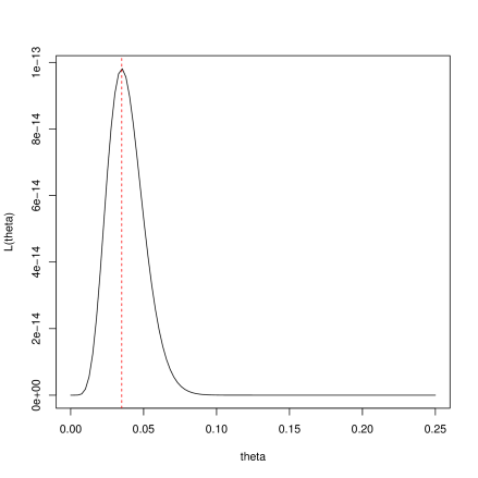
      3. c

         To work out the MLE, we differentiate the (log-)likelihood as usual. The log-likelihood is

         $$l(\theta )=7\log \theta +43\log (1-4\theta ).$$

         Differentiating,

         $$l^{\prime }(\theta )=\frac{7}{\theta }-\frac{4\times 43}{1-4\theta }.$$

         A candidate MLE solves $l^{\prime }(\widehat{\theta })=0$, giving $\widehat{\theta }=\frac{7}{200}$.

         Moreover,

         so this is indeed the MLE.

      4. d

         The observed information is

         	$I_O(\widehat{\theta })$	$=-l^{\prime \prime }(\widehat{\theta })$
         		$={\displaystyle \frac{7}{{\widehat{\theta }}^2}}+{\displaystyle \frac{4\times 4\times 43}{{(1-4\widehat{\theta })}^2}}$
         		$=5714.3+930.2$
         		$=6644.5.$

         So a $95\%$ confidence interval for $\theta$ is

         $$(\widehat{\theta }-\frac{1.96}{\sqrt{I_O(\widehat{\theta })}},\widehat{\theta }+\frac{1.96}{\sqrt{I_O(\widehat{\theta })}})$$

         $$=(0.0110,0.0590).$$

         As $0.02$ is within this confidence interval there is no evidence of this batch being sub-standard.

      14.2 Summary

      {mdframed}

      • 1

        Under certain regularity conditions, the maximum likelihood estimator has, asymptotically, a normal distribution with mean equal to the true parameter value, and variance equal to the inverse of the Fisher information.

      • 2

        The Fisher information is minus the expectation of the second derivative of the log-likelihood evaluated at the true parameter value.

      • 3

        Based on this, we can construct approximate 95% confidence intervals for the true parameter value based on the MLE and the observed information.

      • 4

        Importantly, this is an asymptotic result so is only approximate. In particular, it is a bad approximation to a 95% confidence interval when the sample size, $n$, is small.

      Chapter 15 Deviance and the LRT

      15.1 Deviance-based confidence intervals

      In the last lecture we showed that the MLE is asymptotically normally distributed, and we use this fact to construct an approximate 95% confidence interval.

      In this lecture we will introduce the concept of deviance, and show that this leads to another way to calculate approximate confidence intervals that have various advantages.

      We will begin by showing through an example where things can go wrong with the confidence intervals we know (and love?).

      

      TheoremExample 15.1.1 An evening at the casino

      On a fair (European) roulette wheel there is a $1/37$ probability of each number coming up.

      In the early 1990s, Gonzalo Garcia-Pelayo believed that casino roulette wheels were not perfectly random, and that by recording the results and analysing them with a computer, he could gain an edge on the house by predicting that certain numbers were more likely to occur next than the odds offered by the house suggested. This he did at the Casino de Madrid in Madrid, Spain, winning 600,000 euros in a single day, and one million euros in total.

      Legal action against him by the casino was unsuccessful, it being ruled that the casino should fix its wheel:

      http://en.wikipedia.org/wiki/Roulette#Biased_wheels

      Suppose I am curious that the number 17 seems to come up on a casino’s roulette wheel more frequently than other numbers. I track it for 30 spins, during which it comes up 2 times. I decide to carry out a likelihood analysis on $p$, the probability of the number 17 coming up, and its confidence interval.

      We propose to model the situation as follows. Let $R$ be the number of times the number 17 comes up in 30 spins of the roulette wheel. We decide to model $R\sim \mathrm{Binomial}(30,p)$.

      Why is this a suitable model?

      What assumptions are being made?

      Are these assumptions reasonable?

      The probability of the observed data is given by

      $$\mathrm{Pr}[\text{obs}|p]=\left(\genfrac{}{}{0pt}{}{30}{2}\right)p^2{(1-p)}^{28}.$$

      The likelihood is simply the probability of the observed data, but we can ignore the multiplicative constants, so

      $$L(p)\propto p^2{(1-p)}^{28}.$$

      The log-likelihood is

      $$l(p)=2\log p+28\log (1-p).$$

      Differentiating,

      $$l^{\prime }(p)=\frac{2}{p}-\frac{28}{1-p}.$$

      Now remember solutions to $l^{\prime }(p)=0$ are potential MLEs:

      1. 1

         $\frac{2}{\widehat{p}}=\frac{28}{1-\widehat{p}},$

      2. 2

         $2-2\widehat{p}=28\widehat{p},$

      3. 3

         $\widehat{p}=\frac{2}{30}.$

      The second derivative will both tell us whether this is a maximum, and provide the observed information:

      $$l^{\prime \prime }(p)=-\frac{2}{p^2}-\frac{28}{{(1-p)}^2}.$$

      This is clearly negative for all $p\in (0,1)$, so $\widehat{p}$ must be a maximum.

      Moreover, the observed information is

      	$I_O(\widehat{p})=-l^{\prime \prime }(\widehat{p})$	$={\displaystyle \frac{2}{{\widehat{p}}^2}}+{\displaystyle \frac{28}{{(1-\widehat{p})}^2}}$
      		$=450+32.413$
      		$=482.143.$

      A 95% confidence interval for $p$ is given by

      $$(\widehat{p}-\frac{1.96}{\sqrt{I_O(\widehat{p})}},\widehat{p}+\frac{1.96}{\sqrt{I_O(\widehat{p})}}),$$

      which, on substituting in $\widehat{p}$ and the observed information becomes

      $$(\frac{2}{30}-\frac{1.96}{\sqrt{482.143}},\frac{2}{30}+\frac{1.96}{\sqrt{482.143}})=(-0.023,0.156).$$

      The resulting confidence interval includes negative values (for a probability parameter). What’s the problem??

      Let’s look at a plot of the log-likelihood for the above situation.

      ⬇

      loglik<-function(p){

      2*log(p) + 28*log(1-p)

      }

      p<-seq(from=0.01,to=0.25,length=1000)

      plot(p,loglik(p),type="l")

      

      We notice that the log-likelihood is quite asymmetric. This happens because the MLE is close to the edge of the feasible space (i.e. close to 0). The confidence interval defined above is forced to be symmetric, which seems inappropriate here.

      Definition.

      Suppose we have a log-likelihood function with unknown parameter $\theta$, $l(\theta )$. Then the deviance function is given by

      $$D(\theta )=2\left\{l(\widehat{\theta })-l(\theta )\right\}.$$

      Notice that $D(\theta )\ge 0$, and $D(\widehat{\theta })=0$.

      What can we say about $D(\theta )$?

      This is a fixed (but unknown) value for fixed data $𝐱=x_1,\mathrm{\dots },x_n$. However, in similar spirit to the last lecture, we can consider random data $𝐗=X_1,\mathrm{\dots },X_n$. Now, the deviance function depends on $𝐗$ (since different data leads to different likelihoods). So, $D(\theta ,𝐗)$ is a random variable.

      Theorem 2 (Asymptotic distribution of the deviance).

      Suppose we have an iid sample $\mathrm{X}\mathrm{=}{X}_{\mathrm{1}}\mathrm{,}\mathrm{\dots }\mathrm{,}{X}_n$ from some distribution with unknown parameter $\theta$. Then (under certain regularity conditions) in the limit as $n\mathrm{\to }\mathrm{\infty }$,

      $$D(\theta ,𝐗)\sim {\chi }_1^2,$$

      i.e. the deviance of the true value of $\theta$ has a ${\chi }^{\mathrm{2}}$ distribution with one degree of freedom.

      The practical upshot of this result is that we have another way to construct a confidence interval for $\theta$. A 95% confidence interval for $\theta$, for example, is given by , i.e. any values of $\theta$ whose deviance is smaller than 3.84.

      TheoremExample 15.1.2 An evening at the casino continued

      This property of the deviance is best seen visually. Going back to the roulette data:

      ⬇

      deviance<-function(p){

      2*(loglik(2/30)-loglik(p))

      }

      plot(p,deviance(p),type="l")

      abline(h=3.84)

      

      From the graph we can estimate the confidence interval based on the deviance. In fact the exact answer to three decimal places is $(0.011,0.192)$. Notice that this is not symmetrical, and that all values in the interval are feasible.

      The original motivation for all of this was that we were wondering if the number 17 comes up more often than with the 1/37 that should be observed in a fair roulette wheel.

      In fact 1/37=0.027, which is within the 95% confidence interval calculated above. Hence there is insufficient evidence (so far) to support the claim that this number is coming up more often than it should.

      Notes (summary)

      • 1

        We have now seen two different ways to calculate approximate confidence intervals (CI) for an unknown parameter. Previously, we calculated CI based on the asymptotic distribution of the MLE (CI-MLE). Here, we showed how to calculate the CI based on the asymptotic distribution of the deviance (CI-D).

      • 2

        We discussed various differences and pros and cons of the two:

        1. 1

           CI-MLE is always symmetric about the MLE. CI-D is not.

        2. 2

           CI-MLE can include values with zero likelihood (e.g. infeasible values such as negative probabilities, as seen here). CI-D will only include feasible values.

        3. 3

           CI-D is typically harder to calculate than CI-MLE.

        4. 4

           For reasons we will not go into here, CI-D is typically more accurate than CI-MLE.

        5. 5

           CI-D is invariant to re-parametrization; CI-MLE is not. (This is a good thing for CI-D, that we will learn more about in subsequent lectures).

      • 3

        Overall, CI-D is usually preferred to CI-MLE (since the only disadvantage is that it is harder to compute).

      • 4

        DEVIANCES ARE ALWAYS NON-NEGATIVE!

      15.2 Re-parametrization and Invariance

      TheoremExample 15.2.1 Accident and Emergency continued

      In our likelihood examples we discussed modelling inter-arrival times at an A&E department using an Exponential distribution. The exponential pdf is given by

      $$f(x)=\lambda \exp (-\lambda x)$$

      for $x\ge 0$ and $\lambda \ge 0$, where $\lambda$ is the rate parameter.

      Based on the inter-arrival times (in minutes):

      $$18.39,2.70,5.42,0.99,5.42,31.97,2.96,5.28,8.51,10.90,$$

      giving $\overline{x}=9.259$, we came up with the MLE for $\lambda$ of $\widehat{\lambda }=\frac{1}{\overline{x}}=0.108$.

      Now, $𝔼[X]=\mu =1/\lambda$.

      How would we go about finding an estimate for $\mu$?

      Method 1: re-write the pdf as

      $$f(x)=\frac{1}{\mu }\exp \left(-\frac{x}{\mu }\right),$$

      where $x\ge 0$ and $\mu \ge 0$, to give a likelihood of

      $$L(\mu )=\prod _{i=1}^n\frac{1}{\mu }\exp \left(-\frac{x_i}{\mu }\right),$$

      then find the MLE by the usual approach.

      Method 2: Since $\mu =1/\lambda$, presumably $\widehat{\mu }=1/\widehat{\lambda }=1/0.108=9.259$.

      Which method is more convenient?

      Which method appears more rigorous?

      In fact, both methods give the same solution always. This property is called invariance to reparameterization of the MLE. It is a nice property both because it agrees with our intuition, and saves us a lot of potential calculation.

      Theorem (Invariance of MLE to reparametrisation.).

      If $\widehat{\theta }$ is the MLE of $\theta$ and $\varphi$ is a monotonic function of $\theta$, $\varphi \mathrm{=}g\mathit{}\mathrm{(}\theta \mathrm{)}$, then the MLE of $\varphi$ is $\widehat{\varphi }\mathrm{=}g\mathit{}\mathrm{(}\widehat{\theta }\mathrm{)}$.

      Proof.

      Write $𝐱=(x_1,x_2,\mathrm{\dots },x_n)$. The likelihood for $\theta$ is $L(\theta )=f(\overrightarrow{x}|\theta )$, and for $\varphi$ is $L_{\varphi }(\varphi )$. Note that $\theta =g^{-1}(\varphi )$ as $g$ is monotonic and define $\widehat{\varphi }$ by $g(\widehat{\theta })$. To show that $\widehat{\varphi }$ is the MLE,

      	$L_{\varphi }(\varphi )$	$=f(𝐱|\varphi )$
      		$=f(𝐱|g^{-1}(\varphi ))\le f(𝐱|\widehat{\theta })$

      as $\widehat{\theta }$ is MLE. But

      	$f(𝐱|\widehat{\theta })$	$=f(𝐱|g^{-1}(\widehat{\varphi }))$
      		$=f(𝐱|\widehat{\varphi })=L_{\varphi }(\widehat{\varphi }).$

      ∎

      This means that both methods above must give the same answer.

      Exercise.

      Show this works for the case above, by demonstrating that Method 1 leads to $\widehat{\mu }=\overline{x}=9.259$.

      The following corollary follows immediately from invariance of the MLE to reparametrisation.

      Corollary.

      Confidence intervals based on the deviance are invariant to reparametrisation, in the sense that

      $$\{\varphi :D(g^{-1}(\varphi ))\le 3.84\}=\{\theta :D(\theta )\le 3.84\}.$$

      Proof.

      	$\mathrm{\{}\theta :D(\theta )\le 3.84\}$	$=\{\theta :2(l(\widehat{\theta })-l(\theta ))\le 3.84\}$
      		$=\{\varphi :2(l(g^{-1}(\widehat{\varphi }))-l(g^{-1}(\varphi )))\le 3.84\}$

      by Theorem above, which equals

      $\{\varphi :D(g^{-1}(\varphi ))\le 3.84\}.$

      ∎

      The practical consequence of this is that if

      $({\theta }_l,{\theta }_u)$ is a deviance confidence interval with coverage $p$ for ${\theta }_{\text{𝑡𝑟𝑢𝑒}}$,

      then

      $(g({\theta }_l),g({\theta }_u))$ is a deviance confidence interval with coverage $p$ for ${\varphi }_{\text{𝑡𝑟𝑢𝑒}}$.

      (Of course, $\varphi =g(\theta )$).

      IMPORTANT: This simple translation does not hold for confidence intervals based on the asymptotic distribution to the MLE. This is because that depends on the second derivative of $l(\cdot )$ with respect to the parameter, which will be different in more complicated ways for different parameter choices.

      This will be explored more in MATH330 Likelihood Inference.

      Exam Question

      1. a

         The random variables $X_1,X_2,\mathrm{\dots },X_n$ are independent and identically distributed with the geometric distribution

         $$f(x|\theta )={\theta }^x(1-\theta ),x=0,1,2,\mathrm{\dots }$$

         where $\theta$ is a parameter in the range of $0\le \theta \le 1$ to be estimated. The mean of the above geometric distribution is $\theta /(1-\theta )$.

         1. i

            Write down formulae for the maximum likelihood estimator for $\theta$ and for Fisher’s information;

         2. ii

            Write down what you know about the distribution of the maximum likelihood estimator for this example when $n$ is large.

      2. b

         In a particular experiment, $n=10$, ${\sum }_{i=1}^n{x}_i=10$.

         1. i

            Compute an approximate 95% confidence interval for $\theta$ based on the asymptotic distribution of the maximum likelihood estimator;

         2. ii

            Compute the deviance $D(\theta )$ and sketch it over the range $0.1\le \theta \le 0.9$. Use your sketch to describe how to use the deviance to obtain an approximate 95% confidence interval for $\theta$;

         3. iii

            If you were asked to produce an approximate 95% confidence interval for the mean of the distribution $\theta /(1-\theta )$, what would be your recommended approach? Justify your answer.

      Solution:

      1. a
         1. i

            For the model, the likelihood function is

            	$L(\theta |𝐗)$	$={\displaystyle \prod _{i=1}^n}{\theta }^{X_i}(1-\theta )$
            		$={(1-\theta )}^n{\theta }^{\sum X_i}.$

            The log-likelihood is then

            $$l(\theta |𝐗)=n\log (1-\theta )+\sum X_i\log (\theta ),$$

            with derivative

            $$l^{\prime }(\theta |𝐗)=-\frac{n}{1-\theta }+\frac{\sum X_i}{\theta }.$$

            A candidate MLE solves $l^{\prime }(\widehat{\theta })=0$, giving

            $$\widehat{\theta }=\frac{\sum X_i}{n+\sum X_i}.$$

            Moreover,

            so this is indeed the MLE.

            For the Fisher Information,

            	$I_E(\theta )$	$=𝔼[-l^{\prime \prime }(\theta |𝐗){|}_{\theta =\theta }]$
            		$=𝔼\left[{\displaystyle \frac{n}{{(1-\theta )}^2}}-{\displaystyle \frac{\sum X_i}{{\theta }^2}}\right]$
            		$={\displaystyle \frac{n}{{(1-\theta )}^2}}+{\displaystyle \frac{n}{{\theta }^2}}𝔼[X_1]$
            		$={\displaystyle \frac{n}{{\theta }_{\text{true}}{(1-\theta )}^2}},$

            after simplification, since $𝔼[X_1]=\theta /(1-\theta )$.

         2. ii

            Using the Fisher information, the asymptotic distribution of the MLE is

            $$\widehat{\theta }(𝐗)\sim N({\theta }_{\text{true}},I_E^{-1}({\theta }_{\text{true}}))\approx N({\theta }_{\text{true}},I_0^{-1}(\widehat{\theta })).$$

      2. b
         1. i

            Using the data, the MLE is $\widehat{\theta }=\frac{10}{10+10}=\frac{1}{2}$. The observed information is

            $$I_O(\widehat{\theta })=\frac{10}{{(1-1/2)}^2}+\frac{10}{{(1/2)}^2}=80.$$

            Therefore a $95\%$ confidence interval is

            $$(1/2-\frac{1.96}{\sqrt{80}},1/2+\frac{1.96}{\sqrt{80}})=(0.281,0.719).$$

         2. ii

            The deviance is given by

            	$D(\theta )$	$=2\{l(\widehat{\theta })-l(\theta )\}$
            		$=2\{10\log (1/2)+10\log (1/2)-10\log (1-\theta )-10\log (\theta )\}$
            		$=20\left(-2\log 2-\log (\theta (1-\theta ))\right).$

            To plot the deviance calculate $D(0.1)$ and $D(0.9)$, and note that $D(0.5)=D(\widehat{\theta })=0$. A $95\%$ confidence interval is obtained by drawing a horizontal line at 3.84; the interval is all $\theta$ with $D(\theta )\le 3.84$.

         3. iii

            To construct a confidence interval for the mean, we would use the mean function on the deviance-based confidence interval just calculated, as this is invariant to re-parametrization.

      15.3 Summary

      {mdframed}

      • 1

        The simple, intuitive answer is true: if $\widehat{\theta }$ is a MLE, then if $\varphi =g(\theta )$ for any monotonic transformation $g$, then $\widehat{\varphi }=g(\widehat{\theta })$.

      • 2

        The same simple result can be applied to confidence intervals based on the deviance, but can NOT be applied to confidence intervals based on the asymptotic distribution of the MLE.