Home page for accesible maths 13 Information and Sufficiency 13 Information and Sufficiency 13.2 Suppression of Information

Style control - access keys in brackets

Font (2 3) - + Letter spacing (4 5) - + Word spacing (6 7) - + Line spacing (8 9) - +

13.1 Introduction

Last time we looked at some more examples of the method of maximum likelihood. When the parameter of interest, $\theta$ , is continuous, the MLE, $\hat{\theta}$ , can be found by differentiating the log-likelihood and setting it equal to zero. We must then check the second derivative of the log-likelihood is negative (at our candidate $\hat{\theta}$ ) to verify that we have found a maximum.

Definition.

Suppose we have a sample ${\bf x}=x_{1},\ldots,x_{n}$ , drawn from a density ${f}({\bf x}|\theta)$ with unknown parameter $\theta$ , with log-likelihood $l(\theta|{\bf x})$ . The score function, $S(\theta)$ , is the first derivative of the log-likelihood with respect to $\theta$ :

S(\theta|{\bf x})=l^{\prime}(\theta|{\bf x})=\frac{\partial}{\partial\theta}l(% \theta|{\bf x}).

This is just giving a name to something we have already encountered.

As discussed previously, the MLE solves $S(\hat{\theta})=0$ . Here, $f({\bf x}|\theta)$ is being used to denote the joint density of ${\bf x}=x_{1},\ldots,x_{n}$ . For the iid case, $f({\bf x}|\theta)=\prod_{i=1}^{n}f(x_{i}|\theta)$ . Also, $l(\theta|{\bf x})=\log f({\bf x}|\theta)$ . This is all just from the definitions.

Definition.

Suppose we have a sample ${\bf x}=x_{1},\ldots,x_{n}$ , drawn from a density ${f}({\bf x}|\theta)$ with unknown parameter $\theta$ , with log-likelihood $l(\theta|{\bf x})$ . The observed information function, $I_{O}(\theta)$ , is MINUS the second derivative of the log-likelihood with respect to $\theta$ :

I_{O}(\theta|{\bf x})=-l^{\prime\prime}(\theta|{\bf x})=-\frac{\partial^{2}}{% \partial\theta^{2}}l(\theta|{\bf x}).

Remember that the second derivative of $l(\theta)$ is negative at the MLE $\hat{\theta}$ (that’s how we check it’s a maximum!). So the definition of observed information takes the negative of this to give something positive.

The observed information gets its name because it quantifies the amount of information obtained from a sample. An approximate 95% confidence interval for $\theta_{\text{true}}$ (the unobservable true value of the parameter $\theta$ ) is given by

{\color[rgb]{1,1,1}\left(\hat{\theta}-\frac{1.96}{\sqrt{I_{O}(\hat{\theta})}},% \hat{\theta}+\frac{1.96}{\sqrt{I_{O}(\hat{\theta})}}\right).}

This confidence interval is asymptotic, which means it is accurate when the sample is large. Some further justification on where this interval comes from will follow later in the course.

What happens to the confidence interval as $I_{O}(\hat{\theta})$ changes?

TheoremExample 13.1.1 Mercedes Benz drivers

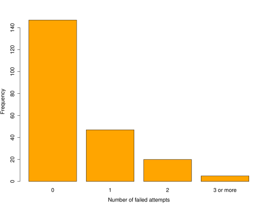
You may recall the following example from last year.The website MBClub UK (associated with Mercedes Benz) carried out a poll on the number of times taken to pass a driving test. The results were as follows.

Number of failed attempts	0	1	2	$\geq 3$
Observed frequency	147	47	20	5

Table 13.1: Number of times taken for drivers to pass the driving test.

As always, we begin by looking at the data.

⬇

obsdata<-c(147,47,20,5)

barplot(obsdata,names.arg=c(0:2, or more'),

xlab="Number of failed attempts",

ylab="Frequency",col="orange")

Next, we propose a model for the data to begin addressing the question.

It is proposed to model the data as iid (independent and identically distributed) draws from a geometric distribution.

Why is this a suitable model?

What assumptions are being made?

Are these assumptions reasonable?

The probability mass function (pmf) for the geometric distribution, where $X$ is defined as the number of failed attempts, is given by

\Pr[X=x]=\theta(1-\theta)^{x},

where $x=0,1,2,\dots$ .

Assuming that the people in the ‘3 or more’ column failed exactly three times, the likelihood for general data $x_{1},\ldots,x_{n}$ is

{\color[rgb]{1,1,1}L(\theta)=\prod_{i=1}^{n}\theta(1-\theta)^{x_{i}},}

and the log-likelihood is

	$\displaystyle l(\theta)$	$\displaystyle=\sum_{i=1}^{n}\log\left\{\theta(1-\theta)^{x_{i}}\right\}$
		$\displaystyle=\sum_{i=1}^{n}\{\log(\theta)+x_{i}\log(1-\theta)\}$
		$\displaystyle=n\log(\theta)+\log(1-\theta)\sum_{i=1}^{n}x_{i}.$

The score function is therefore

{\color[rgb]{1,1,1}S(\theta)=l^{\prime}(\theta)=\frac{n}{\theta}-\frac{\sum_{i% =1}^{n}x_{i}}{1-\theta}.}

A candidate for the MLE, $\hat{\theta}$ , solves $S(\hat{\theta})=0$ :

1

${\color[rgb]{1,1,1}\frac{n}{\hat{\theta}}=\frac{\sum_{i=1}^{n}x_{i}}{1-\hat{% \theta}},}$
2

${\color[rgb]{1,1,1}n(1-\hat{\theta})=\hat{\theta}\sum_{i=1}^{n}x_{i},}$
3

${\color[rgb]{1,1,1}n=\hat{\theta}\left(n+\sum_{i=1}^{n}x_{i}\right),}$
4

${\color[rgb]{1,1,1}\hat{\theta}=\frac{n}{n+\sum_{i=1}^{n}x_{i}}.}$

To confirm this really is an MLE we need to verify it is a maximum, i.e. a negative second derivative.

l^{\prime\prime}(\theta)=-\frac{n}{\theta^{2}}-\frac{\sum_{i=1}^{n}x_{i}}{(1-% \theta)^{2}}<0.

In this case the function is clearly negative for all $\theta\in(0,1)$ , if not we would just need to check this is the case at the proposed MLE.

Now plugging in the numbers, $n=219$ and $\sum_{i=1}^{n}x_{i}=0\times 147+1\times 47+2\times 20+3\times 5=102$ , we get

\hat{\theta}=\frac{219}{219+102}=0.682.

This is the same answer as the ‘obvious one’ from intuition.

But now we can calculate the observed information at $\hat{\theta}$ , and use this to construct a 95% confidence interval for $\theta_{\text{true}}$ .

	$\displaystyle I_{O}(\hat{\theta})$	$\displaystyle=-l^{\prime\prime}(\hat{\theta})$
		$\displaystyle=\frac{n}{\hat{\theta}^{2}}+\frac{\sum_{i=1}^{n}x_{i}}{(1-\hat{% \theta})^{2}}$
		$\displaystyle=\frac{219}{0.682^{2}}+\frac{102}{(1-0.682)^{2}}$
		$\displaystyle=1479.5.$

Now the 95% confidence interval is given by

	$\displaystyle(l,u)$	$\displaystyle=\left(\hat{\theta}-\frac{1.96}{\sqrt{I_{O}(\hat{\theta})}},\hat{% \theta}+\frac{1.96}{\sqrt{I_{O}(\hat{\theta})}}\right)$
		$\displaystyle={\color[rgb]{1,1,1}\left(0.682-\frac{1.96}{\sqrt{1479.5}},0.682+% \frac{1.96}{\sqrt{1479.5}}\right)}$
		$\displaystyle={\color[rgb]{1,1,1}(0.631,0.733)}.$

We should also check the fit of the model by plotting the observed data against the theoretical data from the model (with the MLE plugged in for $\theta$ ).

⬇

#value of theta: MLE

mletheta<-0.682

#expected data counts

expdata<-219*c(dgeom(0:2,mletheta),1-pgeom(2,mletheta))

#make plot

barplot(rbind(obsdata,expdata),names.arg=c(0:2, or more'),

xlab="Number of failed attempts",ylab="Frequency",

col=c("orange","red"),beside=T)

#add legend

legend("topright",c("observed","expected"),

col=c("orange","red"),lty=1)

We can do actually do slightly better than this.

We assumed ‘the people in the “3 or more” column failed exactly three times’. With likelihood we don’t need to do this. Remember: the likelihood is just the joint probability of the data. In fact, people in the “3 or more” group have probability

	$\displaystyle\Pr[X\geq 3]$	$\displaystyle=1-(\Pr[X=0]+\Pr[X=1]+\Pr[X=2])$
		$\displaystyle=1-(\theta+(1-\theta)\theta+(1-\theta)^{2}\theta).$

We could therefore write the likelihood more correctly as

L(\theta)=\prod_{i=1}^{n}\Big{\{}\theta(1-\theta)^{x_{i}}\Big{\}}^{z_{i}}\prod% _{i=1}^{n}\Big{\{}1-(\theta+(1-\theta)\theta+(1-\theta)^{2}\theta)\Big{\}}^{1-% z_{i}},

where $z_{i}=1$ if $x_{i}<3$ and $z_{i}=0$ if $x_{i}\geq 3$ .

NOTE: if all we know about an observation $x$ is that it exceeds some value, we say that $x$ is censored. This is an important issue with patient data, as we may lose contact with a patient before we have finished observing them. Censoring is dealt with in more generality MATH335 Medical Statistics.

What is the MLE of $\theta$ using the more correct version of the likelihood?

The term in the second product (for the censored observations) can be seen as a geometric progression with constant term $a=\theta$ and common ratio $r=(1-\theta)$ , and so $\Pr(X\geq 3|\theta)=(1-\theta)^{3}$ (check that this is the case).

Hence the likelihood can be written

	$\displaystyle L(\theta)$	$\displaystyle=\theta^{n_{u}}(1-\theta)^{\sum x_{i}}\left((1-\theta)^{3}\right)% ^{n_{c}}$
		$\displaystyle=\theta^{n_{u}}(1-\theta)^{\sum x_{i}+3n_{c}}$

where the sum of $x_{i}$ ’s only involves the uncensored observations, $n_{u}$ denotes the number of uncensored observations, and $n_{c}$ is the number of censored observations.

The log-likelihood becomes $l(\theta)=n_{u}\log(\theta)+(\sum x_{i}+3n_{c})\log(1-\theta)$ .

Differentiating, the score function is

S(\theta)=l^{\prime}(\theta)=\frac{n_{u}}{\theta}-\frac{\sum x_{i}+3n_{c}}{1-% \theta}.

A candidate MLE solves $l^{\prime}(\hat{\theta})=0$ , giving

	$\displaystyle\frac{n_{u}}{\hat{\theta}}$	$\displaystyle=\frac{\sum x_{i}+3n_{c}}{1-\hat{\theta}}$
	$\displaystyle n_{u}(1-\hat{\theta})$	$\displaystyle=\hat{\theta}\left(\sum x_{i}+3n_{c}\right)$
	$\displaystyle n_{u}$	$\displaystyle=\hat{\theta}\left(n_{u}+\sum x_{i}+3n_{c}\right)$
	$\displaystyle\hat{\theta}$	$\displaystyle=\frac{n_{u}}{n_{u}+\sum x_{i}+3n_{c}}.$

The value of the MLE using these data is $\frac{214}{214+102}=0.677$ .

Compare this to the original MLE of 0.682.

Why is the new estimate different to this?

Why is the difference small?