Home page for accesible maths 12.4 Likelihood Examples: discrete parameters 12.4 Likelihood Examples: discrete parameters 12.5 Summary

Style control - access keys in brackets

Font (2 3) - + Letter spacing (4 5) - + Word spacing (6 7) - + Line spacing (8 9) - +

Relative Likelihood intervals

The ratio between two likelihood values is useful to look at for other reasons.

Definition.

Suppose we have data $x_{1},\ldots,x_{n}$ , that arise from a population with likelihood function $L(\theta)$ , with MLE $\hat{\theta}$ . Then the relative likelihood of the parameter $\theta$ is

R(\theta)=\frac{L(\theta|{\bf x})}{L(\hat{\theta}|{\bf x})}.

The relative likelihood quantifies how likely different values of $\theta$ are relative to the maximum likelihood estimate.

Using this definition, we can construct relative likelihood intervals which are similar to confidence intervals.

Definition.

A p% relative likelihood interval for $\theta$ is defined as the set

\left\{\theta\left|R(\theta)\geq\frac{p}{100}\right.\right\}.

TheoremExample 12.4.2 Illegal downloads (cont.)

For example a 50% relative likelihood interval for $m$ in our example would be

	$\displaystyle\left\{m\left\|R(m)\geq 0.5\right.\right\}$	$\displaystyle=\left\{m\left\|\frac{0.3^{1}\times 0.7^{m-1}m}{0.3^{1}\times 0.7^% {2}\times 3}\geq 0.5\right.\right\}$
		$\displaystyle=\left\{m\left\|0.7^{m-3}m\geq 1.5\right.\right\}$

By plugging in different values of $m$ , we see that the relative likelihood interval is $\{1,\ldots,7\}$ . The values in the interval can be seen in the figure below.

TheoremExample 12.4.3 Sequential sampling with replacement: Smarties colours

Suppose we are interested in estimating $m$ , the number of distinct colours of Smarties.

In order to estimate $m$ , suppose members of the class make a number of draws and record the colour.

Suppose that the data collected (seven draws) were:

purple, blue, brown, blue, brown, purple, brown.

We record whether we had a new colour or repeat:

New, New, New, Repeat, Repeat, Repeat, Repeat.

Let $m$ denote the number of unique colours. Then the likelihood function for $m$ given the above data is:

L(m|{\bf x_{1}})=1\times\frac{m-1}{m}\times\frac{m-2}{m}\times\frac{3}{m}% \times\frac{3}{m}\times\frac{3}{m}\times\frac{3}{m}.

If in a second experiment, we observed:

New, New, New, Repeat, New, Repeat, New,

then the likelihood would be:

L(m|{\bf x_{2}})=1\times\frac{m-1}{m}\times\frac{m-2}{m}\times\frac{3}{m}% \times\frac{m-3}{m}\times\frac{4}{m}\times\frac{m-4}{m}.

The MLEs in each case are $\hat{m}=3$ and $\hat{m}=8$ .

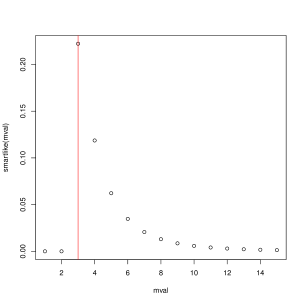
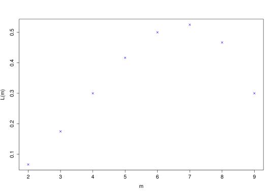
The plots below show the respective likelihoods.

R code for plotting these likelihoods:

⬇

> # experiment 1:

> smartlike<-function(m){

> L<-1*(m-1)*(m-2)*(3)*(3)*(3)*(3)/m^6

> }

> mval<-1:15

> plot(mval,smartlike(mval))

> abline(v=3,col=2)

> which.max(smartlike(mval))

⬇

> # Experiment 2:

> # e.g. pink, purple, blue, blue, brown, purple, orange

> smartlike2<-function(m){

> L<-1*(m-1)*(m-2)*(3)*(m-3)*(4)*(m-4)/m^6

> }

> dev.new()

> plot(mval,smartlike2(mval))

> abline(v=8,col=2)

> which.max(smartlike2(mval))

TheoremExample 12.4.4 Brexit opinions

Three randomly selected members of a class of 10 students are canvassed for their opinion on Brexit. Two are in favour of staying in Europe. What can one infer about the overall class opinion?

The parameter in this model is the number of pro-Remain students in the class, $m$ , say. It is discrete, and could take values $0,1,2,\dots,10$ . The actual true unknown value of $m$ is designated by $m_{\text{true}}$ .

Now $\Pr(\text{obs}|m)$ is

\displaystyle\Pr(\text{2 in favour from $m$ and 1 against from $10-m$}).

Now since the likelihood function of $m$ is the probability (or density) of the observed data for given values of $m$ , we have

	$\displaystyle L(m)$	$\displaystyle=\frac{{m\choose 2}{10-m\choose 1}}{{10\choose 3}}$
		$\displaystyle=\frac{m(m-1)(10-m)}{240}$

for $m=2,3,...,9$ .

This function is not continuous (because the parameter $m$ is discrete). It can be maximised but not by differentiation.

⬇

> #likelihood function

> L<-function(m){

> choose(m,2)*choose(10-m,1)/choose(10,3)

> }

> #values of m to plot

> m<-2:9

> plot(m,L(m),pch=4,col="blue")

The maximum likelihood estimate is $\hat{m}=7.$ Note that the points are not joined up in this plot. This is to emphasize the discrete nature of the parameter of interest.

The probability model is an instance of the hypergeometric distribution.