Home page for accesible maths 12.2 What is likelihood?12.4 Likelihood Examples: discrete parameters

Style control - access keys in brackets

Font (2 3) - + Letter spacing (4 5) - + Word spacing (6 7) - + Line spacing (8 9) - +

12.3 Likelihood Examples: continuous parameters

We now explore examples of likelihood inference for some common models.

TheoremExample 12.3.1 Accident and Emergency

Accident and emergency departments are hard to manage because patients arrive at random (they are unscheduled). Some patients may need to be seen urgently.

Excess staff (doctors and nurses) must be avoided because this wastes NHS money; however, A&E departments also have to adhere to performance targets (e.g. patients dealt with within four hours). So staff levels need to be ‘balanced’ so that there are sufficient staff to meet targets but not too many so that money is not wasted.

A first step in achieving this is to study data on patient arrival times. It is proposed that we model the time between patient arrivals as iid realisations from an Exponential distribution.

Why is this a suitable model?

What assumptions are being made?

Are these assumptions reasonable?

Suppose I stand outside Lancaster Royal Infirmary A&E and record the following inter-arrival times of patients (in minutes):

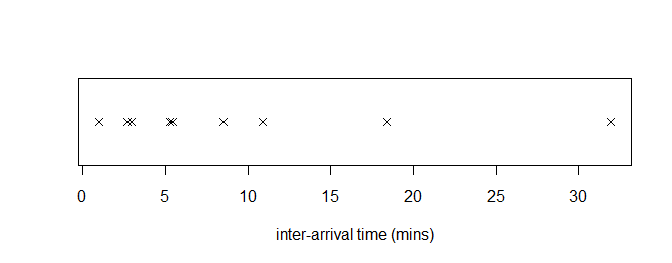
18.39, 2.70, 5.42, 0.99, 5.42, 31.97, 2.96, 5.28, 8.51, 10.90.

As usual, the first thing we do is look at the data!

⬇

arrive<-c(18.39,2.70,5.42,0.99,5.42,31.97,2.96,5.28,8.51,10.90)

stripchart(arrive,pch=4,xlab="inter-arrival time (mins)")

The exponential pdf is given by

f(x)=\lambda\exp(-\lambda x),

for $x\geq 0$ , $\lambda\geq 0$ . Assuming that the data are iid, the definition of the likelihood function for $\lambda$ gives us, for general data $x_{1},\ldots,x_{n}$ ,

{\color[rgb]{1,1,1}L(\lambda)=\prod_{i=1}^{n}\lambda\exp(-\lambda x_{i}).}

Note: we usually drop the ‘ $|{\bf x}$ ’ from $L(\lambda|{\bf x})$ whenever possible.

Usually, when we have products and the parameter is continuous, the best way to find the MLE is to find the log-likelihood and differentiate.

So the log-likelihood is

	$\displaystyle l(\lambda)$	$\displaystyle=\sum_{i=1}^{n}\log\left\{\lambda\exp(-\lambda x_{i})\right\}$
		$\displaystyle=\sum_{i=1}^{n}\left\{\log(\lambda)-\lambda x_{i}\right\}$
		$\displaystyle=n\log(\lambda)-\lambda\sum_{i=1}^{n}x_{i}.$

Now we differentiate:

{\color[rgb]{1,1,1}\frac{\partial}{\partial\lambda}l(\lambda)=l^{\prime}(% \lambda)=\frac{n}{\lambda}-\sum_{i=1}^{n}x_{i}.}

Now solutions to $l^{\prime}(\lambda)=0$ are potential MLEs.

1

${\color[rgb]{1,1,1}\frac{n}{\hat{\lambda}}-\sum_{i=1}^{n}x_{i}=0,}$
2

${\color[rgb]{1,1,1}\hat{\lambda}=\frac{n}{\sum_{i=1}^{n}x_{i}}=\frac{1}{\bar{x% }}.}$

To ensure this is a maximum we check the second derivative is negative:

\frac{\partial^{2}}{\partial\lambda^{2}}l(\lambda)=l^{\prime\prime}(\lambda)=-% \frac{n}{\lambda^{2}}<0.

So the solution we have found is the MLE, and plugging in our data we find (via 1/mean(arrive))

\hat{\lambda}=0.108.

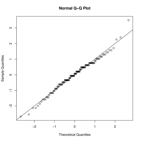
Now that we have our MLE, we should check that the assumed model seems reasonable. Here, we will use a QQ-plot.

⬇

#MLE of lambda (rate)

lam<-1/mean(arrive)

#1/(n+1), 2/(n+1),..., n/(n+1).

quant<-seq(from=1/11,to=10/11,length=10)

#produce QQ-plot

qqplot(qexp(quant,rate=lam),arrive,xlab="Theoretical

quantiles",ylab="Actual")

#add line of equality

abline(0,1)

Given the small dataset, this seems ok – there is no obvious evidence of deviation from the exponential model.

Knowing that the exponential distribution is reasonable, and having an estimate for its rate, is useful to calculate staff scheduling requirements in the A&E.

Extensions of the idea consider flows of patients through the various services (take Math332 Stochastic Processes and/or the STOR-i MRes for more on this).

TheoremExample 12.3.2 Is human body temperature really 98.6 degrees Fahrenheit?

In an article by Mackowiak et al.³³Mackowiak P.A., Wasserman, S.S. and Levine, M.M. (1992) A Critical Appraisal of 98.6 Degrees F, the Upper Limit of the Normal Body Temperature and Other Legacies of Carl Reinhold August Wunderlich, the authors measure the body temperatures of a number of individuals to assess whether true mean body temperature is 98.6 degrees Fahrenheit or not. A dataset of $130$ individuals is available in the normtemp dataset. The data are assumed to be normally distributed with standard deviation $0.73$ .

Why is this a suitable model?

What assumptions are being made?

Are these assumptions reasonable?

What do the data look like?

The plot can be produced using

⬇

> load("normtemp.Rdata")

> hist(normtemp$temperature)

The histogram of the data is reasonable, but there might be some skew in the data (right tail).

The normal pdf is given by

f(x|\mu,\sigma)=\frac{1}{\sqrt{2\pi\sigma^{2}}}\exp\left\{-\frac{(x_{i}-\mu)^{% 2}}{2\sigma^{2}}\right\},

where in this case, $\sigma$ is known.

The likelihood is then

	$\displaystyle L(\mu\|x_{1},\ldots,x_{n})$	$\displaystyle=\prod_{i=1}^{n}\frac{1}{\sqrt{2\pi\sigma^{2}}}\exp\left\{-\frac{% (x_{i}-\mu)^{2}}{2\sigma^{2}}\right\}$
		$\displaystyle=\left(2\pi\sigma^{2}\right)^{-n/2}\exp\left\{-\sum_{i=1}^{n}% \frac{(x_{i}-\mu)^{2}}{2\sigma^{2}}\right\}.$

Since the parameter of interest (in this case $\mu$ ) is continuous, we can differentiate the log-likelihood to find the MLE:

l(\mu)=-\frac{n}{2}\log(2\pi\sigma^{2})-\frac{1}{2\sigma^{2}}\sum_{i=1}^{n}(x_% {i}-\mu)^{2}

and so

l^{\prime}(\mu)=-\frac{1}{2\sigma^{2}}\sum_{i=1}^{n}(-2)(x_{i}-\mu).

For candidate MLEs we set this to zero and solve, i.e.

	$\displaystyle\frac{1}{\sigma^{2}}\sum_{i=1}^{n}x_{i}-n\hat{\mu}$	$\displaystyle=0$
	$\displaystyle\sum_{i=1}^{n}x_{i}-n\hat{\mu}$	$\displaystyle=0$

and so the MLE is $\hat{\mu}=\bar{x}$ .

This is also the “obvious” estimate (the sample mean). To check it is indeed an MLE, the second derivative of the log-likelihood is

l^{\prime\prime}(\mu)=-n<0,

which confirms this is the case.

Using the data, we find $\hat{\mu}=\bar{x}=98.25$ .

This might indicate evidence for the body temperature being different from the assumed 98.6 degrees Fahrenheit.

We now check the fit:

⬇

> temps <-normtemp$temperature # for shorthand

> mean(temps)

[1] 98.24923

> stdtemp = (temps - mean(temps))/0.73

> qqnorm(stdtemp)

> abline(0,1) # add "ideal" fit line y = x

The fit looks good – although (as the histogram previously showed) there is possibly some mild right (positive) skew, indicated by the quantile points above the $y=x$ line.

Why might the QQ-plot show the “stepped” behaviour of the points?

TheoremExample 12.3.3

Every day I cycle to Lancaster University, and have to pass through the traffic lights at the crossroads by Booths (heading south down Scotforth Road). I am either stopped or not stopped by the traffic lights. Over a period of a term, I cycle in 50 times. Suppose that the time I arrive at the traffic lights is independent of the traffic light sequence.

On 36 of the 50 days, the lights are on green and I can cycle straight through. Let $\theta$ be the probability that the lights are on green. Write down the likelihood and log-likelihood of $\theta$ , and hence calculate its MLE.

With the usual iid assumption we see that, if $R$ is the number of times the lights are on green then $R\sim\textrm{Binomial}(50,\theta)$ . So we have

\Pr[R=36]={50\choose 36}\theta^{36}(1-\theta)^{14}.

We therefore have, for general $r$ and $n$ ,

L(\theta)={n\choose r}\theta^{r}(1-\theta)^{n-r},

and

l(\theta)={\color[rgb]{1,1,1}K+r\log(\theta)+(n-r)\log(1-\theta)}.

Solutions to $l^{\prime}(\theta)=0$ are potential MLEs:

l^{\prime}(\theta)={\color[rgb]{1,1,1}\frac{r}{\theta}-\frac{n-r}{1-\theta}},

and if $l^{\prime}(\hat{\theta})=0$ we have

	$\displaystyle\frac{r}{\hat{\theta}}=$	$\displaystyle\ \frac{n-r}{1-\hat{\theta}}$
	$\displaystyle\vspace{.5cm}\mbox{i.e.}\qquad\hat{\theta}=$	$\displaystyle\ \frac{\lx@stackrel{{\scriptstyle\phantom{M}}}{{r}}}{n}.$

For this to be an MLE it must have negative second derivative.

l^{\prime\prime}(\theta)=-\frac{r}{\theta^{2}}-\frac{n-r}{(1-\theta)^{2}}<0.

In particular we have $r=36$ and $n=50$ so $\hat{\theta}=36/50$ is the MLE.

Now suppose that over a two week period, on the 14 occasions I get stopped by the traffic lights (they are on red) my waiting times are given by (in seconds)

4.2,6.9,13.7,2.8,19.3,10.4,1.0,19.4,18.6,0.6,4.5,12.9,0.5,16.0.

Assume that the traffic lights remain on red for a fixed amount of time $t_{r}$ , regardless of the traffic conditions.

Given the above data, write down the likelihood of $t_{r}$ , and sketch it. What is the MLE of $t_{r}$ ?

We are going to assume that these waiting times are drawn independently from $\operatorname{Uniform}[0,t_{r}]$ , where $t_{r}$ is the parameter we wish to estimate.

Why is this a suitable model?

What assumptions are being made?

Are these assumptions reasonable?

Constructing the likelihood for this example is slightly different from those we have seen before. The pdf of the $\operatorname{Uniform}(0,t_{r})$ distribution is

f(x)=\left\{\begin{array}[]{ll}t_{r}^{-1}&\quad 0\leq x\leq t_{r}\\ 0&\quad\text{otherwise}\end{array}\right.

The unusual thing here is that the data enters only through the boundary conditions on the pdf. Another way to write the above pdf is

{\color[rgb]{1,1,1}f(x)=t_{r}^{-1}\mathbf{1}[0\leq x\leq t_{r}],}

where $\mathbf{1}$ is the indicator function.

For data $x_{1},\ldots,x_{n}$ , the likelihood function is then

L(t_{r})={\color[rgb]{1,1,1}\prod_{i=1}^{n}t_{r}^{-1}\mathbf{1}[0\leq x_{i}% \leq t_{r}]}.

We can write this as

	$\displaystyle L(t_{r})$	$\displaystyle=\ t_{r}^{-n}\mathbf{1}\left[\{0\leq x_{1}\leq t_{r}\}\bigcap% \dots\bigcap\{0\leq x_{n}\leq t_{r}\}\right]$
		$\displaystyle=\ t_{r}^{-n}\mathbf{1}[\max(x_{i})\leq t_{r}].$

For our case we have $n=14$ and $\max(x_{i})=19.4$ , so $L(t_{r})=t_{r}^{-14}\mathbf{1}[19.4\leq t_{r}]$ .

We are next asked to sketch this MLE. In R,

⬇

> maxx<-19.4

> #values of t_r to plot

> t<-seq(from=18,to=22,length=1000)

> #likelihood function

> uniflik<-function(t){

> t^(-14)*(t>=19.4)

> }

> plot(t,uniflik(t),type="l")

From the plot it is clear that $\hat{t}_{r}=19.4=\max(x_{i})$ , since this is the value that leads to the maximum likelihood. Notice that solving $l^{\prime}(t_{r})=0$ would not work in this case, since the likelihood is not differentiable at the MLE.

However, on the feasible range of $t_{r}$ , i.e. $\max(x_{i})\leq t_{r}$ , we have

l(t_{r})=-n\log(t_{r}),

and so

l^{\prime}(t_{r})=-n/t_{r}.

Remember that derivatives express the rate of change of a function. Hence since the (log-)likelihood is negative ( $t_{r}>0$ is strictly positive), then the likelihood is decreasing on the feasible range of parameter values.

Since we are trying to maximise the likelihood, this means we should take the minimum over the feasible range as the MLE. The minimum value on the range $\max(x_{i})\leq t_{r}$ is $\hat{t}_{r}=\max(x_{i})=19.4$ .