5.1. Introduction

The material of this section provides some of the most useful mathematical tools available for scientists, engineers, social scientists, and others. We will see how to solve systems of linear equations (see Definition 5.1.2) by using the elementary row operations introduced in Section 2. This technique was used by Chinese mathematicians over two thousand years ago. We will see how to translate a system of linear equations into an augmented matrix, and then row reduce that matrix to solve the equations.

The purpose of the next two examples is to demonstrate what is meant by “solving systems of linear equations”, and to convince you that this is a useful and natural thing to do. These examples show how linear equations may arise in real-life contexts, and we will use them in order to understand a general system of linear equations.

Example 5.1.1.

• Let $y$ be the total cost, in pounds, of producing a certain item and let $x$ be the number of items produced. Suppose that manufacturer A has a start-up cost of £$200$ and a cost per item of £$2$, which gives the equation

  (2)

  $$y=2x+200.$$

  Suppose also that manufacturer B has a start-up price of £$300$ and each item costs £$1.50$, which yields the equation

  (3)

  $$y=\frac{3}{2}x+300.$$

  Which manufacturer should be used?

The equations given by this example are linear, i.e. each variable, here $x$ and $y$, appears with exponent at most one. Also, note that we use the fraction notation $\frac{3}{2}$ instead of the decimal notation $1.5$ in the algebraic equation.

Thus, to answer this question, we start by plotting the two manufacturers’ costs:

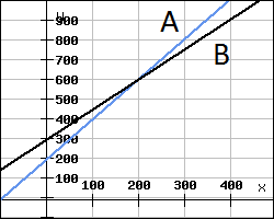
From this diagram, it is clear that the decision depends on the number of items required. Namely, manufacturer A, corresponding to (2), has a lower cost than manufacturer B, as long as the number of items required is less than the $x$-coordinate corresponding to the intersection of the two lines in the graph. This intersection point translates into the fact that both manufacturers’ costs are equal, and we see that to its right, then manufacturer B is cheaper. Thus, we need to find the coordinates of the intersection point. It is given by the values of $x$ and $y$ which simultaneously satisfy Equations (2) and (3).

To find these values, we rearrange the equations in an array, i.e. a matrix, having two rows, say $R_1$ and $R_2$.

We now perform elementary row operations on this “matrix” in order to put it in reduced echelon form. Hence, we first do $R_1=r_1-r_2$ and get new equations

So we deduce that $x=200$. In other words, we perform the row operation $R_1=-2r_1$.

To solve for $y$, we substitute $x$ into $R_2$; in other words we perform $R_2=r_2+\frac{3}{2}{r}_1$:

This is the solution to the system of linear equations. In the terminology of Section 2, we have found the reduced row echelon form of the linear system of equations.

The answer to the original question is that as long as we need no more than $200$ items, then manufacturer A is cheaper than manufacturer B. If we need exactly $200$ items, then both manufacturers will be equally expensive, namely £$600$. Finally, if we need more than $200$ items, manufacturer B is cheaper.

Example 5.1.3.

• The following equations are linear in the variables $x,y,$ and $z$:

  The following equations are not linear in the variables $x,y,$ and $z$:

The coefficients of $x$ and $y$ in the given system of linear equations determine the number of solutions. For instance, let us see see what happens when we slightly modify Example 5.1 by taking the equations

In this case, the graphs are parallel lines, saying that manufacturer A is always cheaper than B.

The geometrical fact that the lines do not intersect corresponds to the algebraic fact that the system of equations has no solution. That is, there are no values of $x$ and $y$ which simultaneously satisfy both equalities, so the system is inconsistent. How can we recognise this situation when there are more than two equations? In the next example we have three equations.

Example 5.1.4.

• Assume an animal’s diet is based on three different types of food A,B and C, where a unit of each one contains the following amount of protein, carbohydrate and fat:

  	protein	carbohydrate	fat
  A	5	3	4
  B	2	2	1
  C	3	1	4

  We require exactly $60$ units of protein, $36$ units of carbohydrate and $50$ units of fat. How many units of A,B and C do we need?

First we translate the word problem into mathematical expressions. The word “exactly” indicates an equality. For instance, counting the amount of protein, we have:

$5\times$ {# units of A} + $2\times$ { # units of B} + $3\times$ { # units of C } $=60$ units.

In order to further translate the problem, let us give names to our variables, say $x,y$ and $z$, for the numbers of units of A,B and C respectively. The above conditions give rise to the following system of linear equations in $x,y$ and $z$.

If we try to proceed as in the first example, we soon run into difficulties, since the equations now represent planes in the three dimensional space. A graphical solution becomes harder to handle by hand. To solve the problem we proceed algebraically by solving the three equations simultaneously for $x,y$ and $z$. Starting from the above array, one way of proceeding is to eliminate variables by using row operations. We eliminate $y$ from $R_1$ and from $R_3$ by doing first $R_3=2r_3-r_1$ and then $R_1=r_1-r_2$. The resulting array is:

Hence, we do $R_1=5r_1-2r_3$, and the new $R_1$ becomes the equation $4x=40$.

From it, we find $x=10$. Now, let us substitute the solution for $x$ into any of the above equations, in order to determine the values of $y$ and $z$. So